All published articles of this journal are available on ScienceDirect.

Sensitivity Analysis and 3D-displacement Inversion of Rock Parameters for High Steep Slope in Open-pit Mining
Abstract
Due to the complexity of multiple rocks and multiple parameters circumstance, various parameters are often reduced to only one parameter empirically to generalize geological conditions, ignoring the really influential parameters. A developed method was presented as a complement to 3D displacement inversion to obtain the relative important parameters under complex conditions with limited computational work. Furthermore, this method was applied to a high steep slope in open-pit mining to investigate field applicability of the developed system. Back analysis was conducted in the reality of the east open-pit working area of Daye Iron Mine and propositional steps were presented for parameters solving in complex circumstance. Firstly, multi-factor and single-factor sensitivity analysis were carried out to classify rock mass and mechanical parameters respectively according to the extent of their effects on deformations. Secondly, based on the results, main influence factors were selected as inversion parameters and taken into a 3D calculating model to get the displacement field and stress field, all of which would be the artificial network training samples together with inversion parameters. Thirdly, taking the real deformations as input for the trained back propagation (BP) neural network, the real material mechanical parameters could be obtained. Finally, the results of trained neural network have been confirmed by field monitoring data and provide a reference to obtain the matter parameters in complicated environment for other similar projects.
1. INTRODUCTION
The rock mass mechanical parameters are the key factors for studying the stability of slope in open-pit mines. Nowadays, the methods and techniques for open-pit slope stability analysis is multifarious, for instance using limit equilibrium methods, numerical methods, probabilistic approaches, etc. [1]. And more recent innovative methods, like Slope Quality Index (SQI) and Rock Engineering Systems (RES) approach incorporate a systemic procedure to estimate slope stability [2].
In the last decades, the numerical method has been applied extensively in current engineering practices to mitigate the complexity and uncertainty of geological factors for a long time. However, the validity in numerical methods is directly or indirectly related to the accuracy of rock mass mechanical parameters of calculations in most practical rock engineering projects.
One powerful approach to tackle this problem is parameter inversion with numerical simulation methods, of which the results were used as the equivalent rock mechanical parameters to reflect something unknown in the whole geotechnical system. Gioda [3] and Sun [4] explored fundamentals principles based on recent developments of the numerical techniques for parameter inversion. Tang et al. [5] published systematical treatise about engineering geology numeral simulation and back analysis of parameters. Levasseur et al. [6] set out the identification of constitutive parameters from in-situ geotechnical measurements. Kveldsvik [7] and Cai [8] back-calculated rock mass strength parameters based on measured displacements and geotechnical data. Li et al. [9] experienced how the equivalent parameters obtained and affected the estimates of safety factors.
Scholars presented practical new methods and obtained a practically unique solution for the elasto-plastic back analysis for rock mechanical parameters [10-12]. Artificial neural network (ANN) and genetic algorithm were also applied to parameters inversion to get the optimized solution of mechanical parameters in recent years [13-16], and typical examples were given in different circumstances to prove the feasibility and accuracy, such as powerhouse cavern [17, 18], large landslides [19], excavation support systems [20], sequential tunneling [21, 22], complex rock slope deformation [23-25].
The essential restriction of parameter inversion is that the parameters of compute should be established at the outset: if do not know the purpose of the study, we cannot determine which variables are relevant. So, when there are different types of rocks in the studying area, scholars often simplify geological conditions and select only one of those various parameters or formations according to their project experience. Yet amid to simplify calculations, there are concerns that the reductionist approach is poorly precise and even fail to serve its purpose. For mining excavation calculation in particular, big area coverage, long excavating cycle, there are very complex overlying strata and mechanical parameters of rock mass involved in calculation, the hypothesis of singular one media or excavating all at once cannot satisfy the needs of engineering.
Despite the existence of back-analysis, a more complete one that is able to combine a broader number of potential relevant factors and parameters of complex rock engineering projects is still lacking. Thereby, in this paper, a newly approach that integrates the features of 3 dimensional (3D) displacement inversion and sensitivity analysis was developed to infer the uncertainties under complex geological conditions from a holistic point of view and obtain the really matter sensitive parameters with finite calculations, and the east open-pit working area of Daye Iron Mine in China were selected as the case study examples.
2. METHODOLOGY
As far as a practical mining excavation calculation model, the complex nonlinear relationship between the characteristic factors of rocks and their mechanical behaviors by explicit functions may be unquantifiable. Once all the potentially relevant relations have to been taken into account, the given parameters of compute will be enormous and more difficult to determine. A new and simplified approach developed from 3D-displacement inversion is presented for the determination of rock mechanics parameters, to this system, multi-factor sensitivity analysis and mono-factor sensitivity analysis are added to improve it. Fig. (1) illustrates the flow chart of this study.
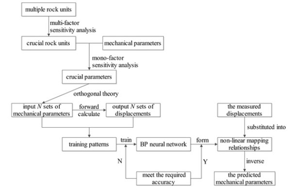
The flow chart of the improved inversion method.
The major steps for obtaining rock parameters are organized as follows:
- When the 3D numerical calculation model of study area have been established, all rock units in the area should be ranked firstly by multi-factor sensitivity analysis according to their influence on the deformation of 3D numerical model.
- Then sort the mechanical parameters of the relative important rocks in terms of vulnerability to ground deformation by mono-factor sensitivity analysis. After the relative importance of each rock units and mechanical parameters determined, the parameters with larger weights will be chosen as inversion parameters for computing.
- Take the inversion parameters (E, μ, C, φ et al.) into 3D numerical model to calculate the displacement field and stress field (σ, u), both the two sets of data, the inversion parameters and numerical results (σ, u)), make up the training samples for artificial neural network (ANN).
- When the training is completed from the training samples, the well-trained neural network could excellent map the nonlinear relation between parameters and numerical results. And then input the measured displacement (u*) into the trained network as predicting sample to obtain the real material parameters (E*, μ*, C*, φ* et al).
- Apply the real material parameters (E*, μ*, C*, φ*et al.) into 3D model, and the stress and the displacement deformation are obtained from the forward calculation results, which are verified by the field monitoring data to ensure the accuracy of parameters.
The results can meet the requirement of the project and provide a theoretical basis for long-term stability of super high steep slopes.
3. PRACTICAL APPLICATIONS
3.1. Sampling Location and 3D Model
Fig. (2) shows the aerial photo of Daye Iron Mine and the open-pit slope. The East Pit of Daye Iron Mine is 2.4 km long in E-W direction and 1.0 km long in S-N direction. The height of north slope of Daye open-pit is within 170~270 m and that of the south slope is within 86~200 m. The high-steep slope here is 230~430 m high and the slope angle varies between 38° and 43°. Open pit method is adopted. Fig. (3) shows the location of the selected study area in the East Pit of Daye Iron Mine.
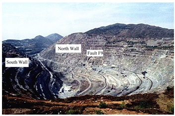
The aerial photo of Daye Iron Mine and the open-pit slope.
The study area’s geological structure is medially developed. Most rock masses are jointed solid rock, and there are two main faults: F9 and F25, both of which pass through the upper bed and the lower bed respectively. The in-situ stress test results indicate that no remarkable tectonic stress appears.
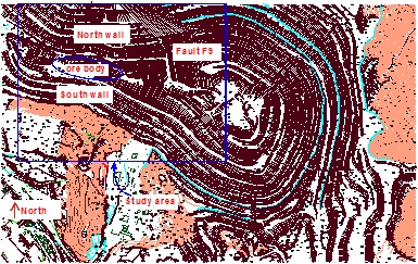
Location of the selected study area (inside the blue rectangle) in the East Pit of Daye Iron Mine.
Mohr-Coulomb (M-C) model was considered as the material model for numerical simulation [26]. Considering the stress elimination, the model size’s in the E-W, N-S, and vertical direction was 900 m, 800 m and 680 m. The study areas can be divided into five rock units: diorite, marble, magnetite, fault fracture zone and back filled body according to the type of rock masses. Tetrahedral meshes were used in the model, and composed of 76331 elements and 131016 nodes. Fig. (4) shows the 3D numerical calculation model.
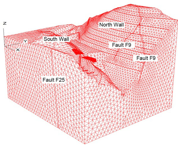
Finite difference grid and 3D numerical calculation model.
In this calculation, five subsidence checkpoints were selected to process sensitively analysis. Checkpoints are represented by one of these letters U1, U2, U3, U4, U5, these letters correspond to locations south slope-diorite, north slope-marble, back filled body group, magnetite group and fault fracture zone, respectively.
3.2. Factors Definition with Sensitivity Analysis
According to the related investigation data and the preliminary research results [27], parameter values in Table 1 were regarded as the reference values for sensitivity analysis. 25 vast and complex different rock parameters need to be considered in the studying area. If every parameter of each rock units needed to be inverted, the number of combined schemes could be significantly large. Besides, output variables’ number is too great to get each parameter accurately. For that, some measures, namely multi-factor and mono-factor sensitivity analysis, are taken to achieve less parameters and definite solution.
Reference values for sensitivity analysis model.
| Rock units | Elasticity modulus /GPa |
Poisson’s ratio |
Cohesion /MPa |
Internal friction angle /(°) |
Tensile strength /MPa |
|---|---|---|---|---|---|
| Marble | 8.5 | 0.23 | 0.26 | 30 | 0.25 |
| Diorite | 9.0 | 0.23 | 0.27 | 29 | 0.10 |
| Magnetite | 7.8 | 0.27 | 0.35 | 42 | 0.35 |
| Back filled body | 3.0 | 0.22 | 0.07 | 27 | 0.02 |
| Fault fracture zone | 3.0 | 0.22 | 0.30 | 22 | 0.04 |
3.2.1. Multi-factor Sensitivity Analysis of Rocks
Rocks should be firstly ranked by multi-factor sensitivity analysis according to their influence on deformation. In the part, factors were the five rock units, based on the reference values in Table 1, four levels (i=1, 2, 3, 4) were chosen: the reference value, reference value rise by 20%, reference value rise by 10%, reference value fall by 10%. Table 2 shows the 5-factor 4-level orthogonal experiment (L16(45)) and the corresponding results of multi-factor sensitivity analysis.
The orthogonal table and results.
| No. | Factors and levels of orthogonal experiment | ||||
|---|---|---|---|---|---|
| Marble | Diorite | Magnetite | Back filled body | Fault fracture zone | |
| 1 | 1 | 1 | 1 | 1 | 1 |
| 2 | 1 | 2 | 2 | 2 | 2 |
| 3 | 1 | 3 | 3 | 3 | 3 |
| 4 | 1 | 4 | 4 | 4 | 4 |
| 5 | 2 | 1 | 2 | 3 | 4 |
| 6 | 2 | 2 | 1 | 4 | 3 |
| 7 | 2 | 3 | 4 | 1 | 2 |
| 8 | 2 | 4 | 3 | 2 | 1 |
| 9 | 3 | 1 | 3 | 4 | 2 |
| 10 | 3 | 2 | 4 | 3 | 1 |
| 11 | 3 | 3 | 1 | 2 | 4 |
| 12 | 3 | 4 | 2 | 1 | 3 |
| 13 | 4 | 1 | 4 | 2 | 3 |
| 14 | 4 | 2 | 3 | 1 | 4 |
| 15 | 4 | 3 | 2 | 4 | 1 |
| 16 | 4 | 4 | 1 | 3 | 2 |
| S1 | 330.5 | 153.5 | 265.7 | 291.9 | 310.5 |
| S2 | 305.25 | 6.9 | 284.9 | 305.7 | 277.7 |
| S3 | 283.35 | 34.3 | 313.7 | 270.65 | 294.55 |
| S4 | 280.7 | 1005 | 335.3 | 331.45 | 317.4 |
| X1 | 82.625 | 38.375 | 66.43 | 72.975 | 77.625 |
| X2 | 76.312 | 1.725 | 71.22 | 76.425 | 69.425 |
| X3 | 70.837 | 8.575 | 78.42 | 67.662 | 73.637 |
| X4 | 70.175 | 251.25 | 83.83 | 82.862 | 79.35 |
| R | 12.45 | 249.52 | 17.4 | 15.2 | 9.925 |
Xi (i=1,2,3,4): average value of the sum of four computational displacements, Xi = Si/ 4;
R: the range of Xi, R=Xmax-Xmin;
Levels (i=1, 2, 3, 4): the reference value, reference value rise by 20%, reference value rise by 10%, reference value fall by 10%.
For several factors simultaneously changed were considered. The range of the average value of factors (R) could reflect the differences of sensibility of the factors accurately. Analyzed the range ‘R’ of each factor in Table 2 and assessed affecting degree of each rock unit were diorite, magnetite, the back filled body, marble, and faults. These results were in coincidence with previous practical project experience.
3.2.2. Mono-factor Sensitivity Analysis of Parameters
The mono-factor sensitivity analysis was applied to rank the relative importance of mechanical parameters of each single type of rock mass. Firstly, 5 mechanical parameters of each rock mass (listed in Table 1) were taken as the fundamental state, U = f (x1, x2, x3, ...xn). When the other entire parameters are fixed, the parameter xi varied at a time with increasing by 20%, increasing by 10%, and reducing by 10%. If a small change of factor X in the inputs could produce the greatest effects on output U, then the displacements of monitoring points U was marked sensitive to the changes in factor xi.
The overall parameters of the rock units are presented and for one specific rock mass, the diorite, the calculation of mono-factor sensitivity is presented in detail. The 5 mechanical parameters values (Table 1) were considered as base values and reasonably compounded in the calculation table of mono-factor sensitivity analysis to obtain the displacements U as shown in Table 3.
Calculation table of mono-factor sensitivity analysis of diorite.
| No. |
Elasticity modulus /GPa |
Poisson’s ratio |
Cohesion /MPa |
Internal friction angle /(°) | Tensile strength /MPa |
U1 /mm |
U2 /mm |
U3 /mm |
U4 /mm |
|---|---|---|---|---|---|---|---|---|---|
| 1 | 9.00 | 0.23 | 0.27 | 29.00 | 0.10 | 52.00 | 2.20 | 12.94 | 0.99 |
| 2 | 10.80 | 0.23 | 0.27 | 29.00 | 0.10 | 43.00 | 1.80 | 10.55 | 0.76 |
| 3 | 9.90 | 0.23 | 0.27 | 29.00 | 0.10 | 47.00 | 2.00 | 11.49 | 0.81 |
| 4 | 8.10 | 0.23 | 0.27 | 29.00 | 0.10 | 57.80 | 2.40 | 14.56 | 1.12 |
| 5 | -- | -- | -- | -- | -- | -- | -- | -- | -- |
| 6 | 9.00 | 0.28 | 0.27 | 29.00 | 0.10 | 48.00 | 2.85 | 13.18 | 1.77 |
| 7 | 9.00 | 0.25 | 0.27 | 29.00 | 0.10 | 52.00 | 2.50 | 13.73 | 1.40 |
| 8 | 9.00 | 0.21 | 0.27 | 29.00 | 0.10 | 51.00 | 1.96 | 14.28 | 0.60 |
| 9 | -- | -- | -- | -- | -- | -- | -- | -- | -- |
| 10 | 9.00 | 0.23 | 0.32 | 29.00 | 0.10 | 30.50 | 1.45 | 12.89 | 2.14 |
| 11 | 9.00 | 0.23 | 0.30 | 29.00 | 0.10 | 39.50 | 1.75 | 12.46 | 1.62 |
| 12 | 9.00 | 0.23 | 0.24 | 29.00 | 0.10 | 69.50 | 2.82 | 14.49 | 0.68 |
| 13 | -- | -- | -- | -- | -- | -- | -- | -- | -- |
| 14 | 9.00 | 0.23 | 0.27 | 34.80 | 0.10 | 9.20 | 1.33 | 14.25 | 4.13 |
| 15 | 9.00 | 0.23 | 0.27 | 31.90 | 0.10 | 24.00 | 1.60 | 12.93 | 2.65 |
| 16 | 9.00 | 0.23 | 0.27 | 26.10 | 0.10 | 158.00 | 3.50 | 16.24 | 1.70 |
| 17 | -- | -- | -- | -- | -- | -- | -- | -- | -- |
| 18 | 9.00 | 0.23 | 0.27 | 29.00 | 0.12 | 52.50 | 2.25 | 14.02 | 0.85 |
| 19 | 9.00 | 0.23 | 0.27 | 29.00 | 0.11 | 52.20 | 2.23 | 13.35 | 1.03 |
| 20 | 9.00 | 0.23 | 0.27 | 29.00 | 0.09 | 51.90 | 2.17 | 12.91 | 0.98 |
Ui is the displacements of four checkpoints computed by numerical calculation model. U1, U2, U3, U4, U5, correspond to locations south slope-diorite, north slope-marble, back filled body group, magnetite group and fault fracture zone, respectively.
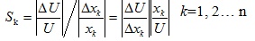
For a quantitative comparison, the original combination indicators should be transformed into comparable values by the dimensionless method. Sensitivity of a normalized parameter was defined by the following formula [28]:
 |
(1) |
where Sk is the sensitivity of factor xk,
 is the relative variation of displacements; and
 is the relative variation of a given factor.
Plug mechanical parameters (Table 3) into the equation, then sensitivities of diorite’s factors were calculated as the ‘U1’ in Table 4. The sensitivity coefficients stand for the relative importance of mechanical parameters of diorite. Three factors were separated from the five mechanical parameters: internal friction angle (9.9615), cohesion (2.6122), and elasticity modulus (0.9817).
Sensitivity coefficients of each position’s mechanical parameters.
| Monitoring points |
Elasticity modulus /GPa |
Poisson’s ratio |
Cohesion /MPa |
Internal friction angle /(°) |
Tensile strength /MPa |
|---|---|---|---|---|---|
| U1 | 0.9807 | 0.2115 | 2.6122 | 9.9615 | 0.0353 |
| U2 | 0.9091 | 1.3106 | 2.1894 | 3.5379 | 0.1288 |
| U3 | 1.0995 | 0.5796 | 0.245 | 1.0211 | 0.5059 |
| U4 | 1.0746 | 4.0122 | 5.1041 | 19.6870 | 0.4133 |
Similar to the exception of diorite, sensitivity coefficients of all the five monitoring positions’ mechanical parameters were obtained as listed in Table 4. The sampling schemes for inversion are, in fact the parameter combinations of finite element calculation, and elasticity modulus are mandatory. According to the sensitivity coefficients, 11 parameters that have relatively larger impact on slope deformations were showed in descending orders are as follows:
U1: Diorite in north slope: internal friction angle, cohesion, elasticity modulus;
U2: Marble in south slope: internal friction angle, cohesion, elasticity modulus;
U3: The back filled body: elasticity modulus, internal friction angle ;
U4: Magnetite: internal friction angle, cohesion, elasticity modulus.
With a view to the specificity of fault fracture zone, the following parameters were also chosen as the target vectors:
Faults: internal friction angle, cohesion, elasticity modulus.
Consequently there are a total of 14 pivotal parameters selected from 25 mechanical parameters to be calculated.
Orthogonal design table for 14 levels of factor 2.
| No. | Levels | ||||||||||||||
|---|---|---|---|---|---|---|---|---|---|---|---|---|---|---|---|
| X1 | X2 | X3 | X4 | X5 | X6 | X7 | X8 | X9 | X10 | X11 | X12 | X13 | X14 | X15 | |
| 1 | 1 | 1 | 1 | 1 | 1 | 1 | 1 | 1 | 1 | 1 | 1 | 1 | 1 | 1 | |
| 2 | 1 | 1 | 1 | 1 | 1 | 1 | 1 | 2 | 2 | 2 | 2 | 2 | 2 | 2 | |
| 3 | 1 | 1 | 1 | 2 | 2 | 2 | 2 | 1 | 1 | 1 | 1 | 2 | 2 | 2 | |
| 4 | 1 | 1 | 1 | 2 | 2 | 2 | 2 | 2 | 2 | 2 | 2 | 1 | 1 | 1 | |
| 5 | 1 | 2 | 2 | 1 | 1 | 2 | 2 | 1 | 1 | 2 | 2 | 1 | 1 | 2 | |
| 6 | 1 | 2 | 2 | 1 | 1 | 2 | 2 | 2 | 2 | 1 | 1 | 2 | 2 | 1 | |
| 7 | 1 | 2 | 2 | 2 | 2 | 1 | 1 | 1 | 1 | 2 | 2 | 2 | 2 | 1 | |
| 8 | 1 | 2 | 2 | 2 | 2 | 1 | 1 | 2 | 2 | 1 | 1 | 1 | 1 | 2 | |
| 9 | 2 | 1 | 2 | 1 | 2 | 1 | 2 | 1 | 2 | 1 | 2 | 1 | 2 | 1 | |
| 10 | 2 | 1 | 2 | 1 | 2 | 1 | 2 | 2 | 1 | 2 | 1 | 2 | 1 | 2 | |
| 11 | 2 | 1 | 2 | 2 | 1 | 2 | 1 | 1 | 2 | 1 | 2 | 2 | 1 | 2 | |
| 12 | 2 | 1 | 2 | 2 | 1 | 2 | 1 | 2 | 1 | 2 | 1 | 1 | 2 | 1 | |
| 13 | 2 | 2 | 1 | 1 | 2 | 2 | 1 | 1 | 2 | 2 | 1 | 1 | 2 | 2 | |
| 14 | 2 | 2 | 1 | 1 | 2 | 2 | 1 | 2 | 1 | 1 | 2 | 2 | 1 | 1 | |
| 15 | 2 | 2 | 1 | 2 | 1 | 1 | 2 | 1 | 2 | 2 | 1 | 2 | 1 | 1 | |
| 16 | 2 | 2 | 1 | 2 | 1 | 1 | 2 | 2 | 1 | 1 | 2 | 1 | 2 | 2 | |
X4: elasticity modulus of marble; X5: cohesion of marble; X6: internal friction angle of marble;
X7: elasticity modulus of magnetite; X8: cohesion of magnetite; X9: internal friction angle of magnetite; X10: elasticity modulus of the fault fracture zone; X11: cohesion of the fault fracture zone; X12: internal friction angle of the fault fracture zone; X13: elasticity modulus of the back filled body; X14: internal friction angle of the back filled body; X15: null.
Level 1 and 2: represent reference value rise by 10% and fall by 10%.
3.3. Mechanical Parameters Inversion with Neural Network
3.3.1. Training Samples of Neural Network
The 14 acquired key parameters and a “null” were taken as 15 factors, and each factor was divided into 2 value levels, namely each factor represent 110% and 90% of the baseline value respectively. Then, a orthogonal experiment design (L16(215)) was applied (Table 5), of which the combined projects {X1i, X2i, X3i, ...X15i }, i = 16 were regard as output vector.
Numerical tests of these combined projects were carried out with the 3D model (Fig. 4), the displacements of the five representative positions in different situations were calculated (listed in Table 6), and regard as the input vector.
Displacement deformation of analysis model.
| No. | U1 | U2 | U3 | U4 | U5 |
|---|---|---|---|---|---|
| 1 | -1.590 | -2.508 | 0.010 | 0.068 | 0.248 |
| 2 | -2.469 | -3.308 | 0.040 | 0.032 | 0.276 |
| 3 | -2.842 | -4.002 | 0.000 | 0.045 | 0.257 |
| 4 | -2.634 | -3.646 | -0.010 | 0.060 | 0.169 |
| 5 | -8.311 | -9.802 | -0.018 | 0.021 | 0.195 |
| 6 | -89.180 | -105.100 | -0.025 | -0.048 | 0.201 |
| 7 | -88.410 | -104.800 | -0.014 | 0.028 | 0.294 |
| 8 | -89.750 | -104.700 | -0.032 | 0.022 | 0.185 |
| 9 | -42.930 | -49.210 | -0.014 | 0.030 | 0.231 |
| 10 | -41.870 | -48.250 | -0.014 | 0.044 | 0.234 |
| 11 | -44.970 | -52.140 | -0.017 | 0.042 | 0.228 |
| 12 | -43.240 | -49.610 | 0.002 | 0.020 | 0.234 |
| 13 | -8.293 | -9.799 | 0.013 | 0.067 | 0.372 |
| 14 | -9.402 | -11.210 | 0.058 | 0.070 | 0.267 |
| 15 | -8.628 | -10.280 | 0.050 | 0.075 | 0.269 |
| 16 | -8.347 | -9.874 | 0.070 | 0.054 | 0.580 |
U3: checkpoint allocated in back filled body group; U4: checkpoint allocated in magnetite group.
U5: checkpoint allocated in fault fracture zone.
By now, the training samples for neural network were acquired completely.
3.3.2. Neural Network Training
(1) Artificial neural network (ANN) design
The ANN model used here is based on the standard BP network architecture, which consists of fully interconnected layers of processing units, incorporated with transfer functions [29].
-
Input and output layer
The number of input neurons and output neurons depended on the number of elements in BP network. Input neurons were the displacements on 5 representative points and output neurons were 14 mechanical parameters, so a 5-input, 14-output network was necessary. -
Hidden layer
A network with multiple hidden neurons can approximate any nonlinear multidimensional function. To improve the computation efficiency, one hidden layer was selected to form the network. Deciding the number of neurons in the hidden layers was a very important part of deciding the overall neural network architecture. Using too few neurons in the hidden layers will result in something called under-fitting. Under-fitting can lead to no convergence. Using too many neurons in the hidden layers can result in over-fitting. An inordinately large number of neurons in the hidden layers can also increase the time it takes to train the network. The amount of training time can increase to the point that it is impossible to adequately train the neural network. Obviously, some compromise must be reached between too many and too few neurons in the hidden layers. Generally, the number of hidden neurons can be decided in following formula [30]:
(2) where n1 is the number of hidden neurons; n is the number of output neurons, and n=5; m is the number of input neurons, and m=14; a is a constant ranging from 1 to 10. Calculations indicate that the number of hidden neurons ranges between 5 and 15.
(3) -
The modified BP algorithm
The Neural Network Toolbox provided tools for designing, implementing, visualizing, and simulating neural networks. Existing functions in MATLAB were called to implement the BP algorithms and the modified BP algorithms. A log-sigmoid transfer function (Logsig) was used to calculate the hidden layer’s output, and a linear transfer function (Purelin) was employed to calculate the output layer’s output.
(2) Training the network
Based on the relative research achievements and engineering experiences, n1=6, n1=9 and n1=12 were selected as the numbers of hidden neurons. The data listed in Tables 5 and 6 were imported into the network as training samples. In the training process, the network prediction error went down incrementally until it fell below 10-4, Fig. (5) shows the diagram of the considered BP network in the learning stage.
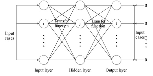
Diagram of the considered BP network in the learning stage.
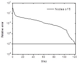
Error curve for 6 nodes network structure.
Figs. (6-8) show the errors decrease with increasing epochs when n1=6, n1=9 and n1=12 respectively. Results showed that the network with 9 hidden neurons performed better than others and could meet the requirement of accuracy.
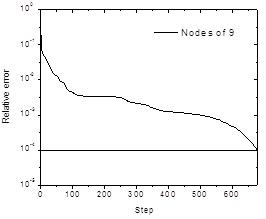
Error curve for 9 nodes network structure.
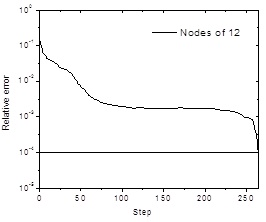
Error curve for 12 nodes network structure.
3.3.3. Inverse Analysis of Mechanical Parameters
Once the ANN has been trained using the training set, the interaction function can be established with the non-linear function between mechanical parameters and displacements. The actual displacements of five monitoring points: U0= [-35, -163, 0.75, -3.65, 1.12] (units: mm) was imported as the given input for the network with 9 hidden neurons. Then the output vectors would be the predicted mechanical parameters, as listed in Table 7.
Rock mechanics parameters determined by back analysis.
| Petrofabrics | Modulus of elasticity /GPa |
Poisson’s ratio |
Cohesion /MPa |
Internal friction angle /(°) |
Tensile strength /MPa |
|---|---|---|---|---|---|
| Marble | 15.60 | 0.23 | 0.25 | 28 | 0.25 |
| Diorite | 16.90 | 0.23 | 0.26 | 30 | 0.10 |
| Magnetite | 12.50 | 0.27 | 0.35 | 40 | 0.35 |
| Back filled body | 2.00 | 0.20 | 0.07 | 27 | 0.02 |
| Fault fracture zone | 1.70 | 0.20 | 0.13 | 23 | 0.04 |
3.4. Field Test Verification
The mechanical parameters calculated by inversion have great practical value in the surrounding rock stability and the slope stability of open-pit. The obtained parameters in Table 7 were applied to simulate open-pit excavation. Monitoring points F9-5 and F9-6 are located on both sides of Fault F9. Both the calculated vertical and horizontal displacements were compared with the field monitoring data to verify the the accuracy of the network. As listed in Table 8, the maximum error rate between numerically simulated data and field monitoring data was 13%, and the minimum error rate was as low as 0.2%. The basic agreement of those two sets of data indicates that the mechanical parameters and initial stress field obtained from the proposed back analysis are reasonable.
Observational and computational results comparison.
| No. |
Observational data /mm |
Computational results /mm |
Relative error | |
|---|---|---|---|---|
| F9-6 | Z-Displacement | 35.0 | 34.5 | 1.4% |
| X-Displacement | 27.0 | 30.7 | 13.0% | |
| F9-5 | Z-Displacement | 149.0 | 143.1 | 3.9% |
| X-Displacement | 112.0 | 112.2 | 0.2% | |
Verification analysis shows good agreements between the simulation results and the actual field data for slope stability in open-pit mines. As discussed in relation to the project example, this developed method could cull the pivotal parameters from amount of parameters correctly and effectively, and has good field applicability, not only for slope stability, but other rock engineering projects with complicated geological conditions.
CONCLUSION
- Both multi-factor sensitivity analysis and mono-factor sensitivity analysis were employed to determine the influence of rock types and mechanical parameters. In descending order, the lists of material types according their influence on slope deformations were diorite, magnetite, the back filled body, marble and the faults, which in coincidence with previous practical project experience. In descending order, the lists of mechanical parameters according their influence on slope deformations were internal friction angle, cohesion, elastic modulus, poisson ratio and tensile strength.
- Take the obtained parameters into the 3D calculation model, the results showed that the small relative errors between numerical simulation result and the observation data meet the requirement of precision. So the 3D-displacement inversion with sensitivity analysis had great value in engineering applications of multi-parameters and provided a theoretical basis for long-term stability of super high steep slopes.
- The method presented in this paper is a natural development of 3D displacement inversion, rock mechanical parameters could be successfully predicted and reliable for further study with finite steps. Improved by both multi-factor sensitivity analysis and mono-factor sensitivity analysis, this method could screen out the most efficacious rock mechanical parameters correctly and reasonably in complex environment with simple calculations. Furthermore, 5 reference detailed calculating steps were provided for parameter inversion in multiple rocks and multiple parameters circumstance.
CONFLICT OF INTEREST
The authors confirm that this article content has no conflict of interest.
ACKNOWLEDGEMENTS
The authors would like to acknowledge the financial support of the National Natural Science Foundation of China (Grant No. 41372312, No. 41072219) and the China Scholarship Council (CSC), and the Fundamental Research Funds for the Central Universities, China University of Geosciences (Wuhan) (Grant No.CUGL140817) for financial support. The authors would like to express sincere thanks to the reviewers for their constructive comments.