All published articles of this journal are available on ScienceDirect.

Revised Level Set-Based Method for Topology Optimization and Its Applications in Bridge Construction
Abstract
To cure imperfections such as low accuracy and the lack of ability to nucleate hole in the conventional level set-based topology optimization method, a novel method using a trapezoidal method with discrete design variables is proposed. The proposed method can simultaneously accomplish topology and shape optimization. The finite element method is employed to obtain element properties and provide data for calculating design and topological sensitivities. With the aim of performing the finite element method on a non-conforming mesh, a relation between the level set function and the element densities field has to be clearly defined. The element densities field is obtained by averaging the Heaviside function values. The Lagrange multiplier method is exploited to fulfill the volume constraint. Based on topological and design sensitivity and the trapezoidal method, the Hamilton-Jacobi partial differential equation is updated recursively to find the optimal layout. In order to stabilize the iterations and improve the efficiency of the algorithm, re-initiation of the level set function is necessary. Then, the detailed process of a cantilever design is illustrated. To demonstrate the applications of the proposed method in bridge construction, two numerical examples of a pylon bridge design are introduced. It is shown that the results match practical designs very well, and the proposed method is a helpful tool in bridge design.
1. INTRODUCTION
Topology optimization is conducive to the conceptual design of a structure and enables engineers to find optimal material distribution. A wide range of fascinating applications of topology optimization has been developed [1-3]. Sophisticated methods have emerged to help engineers deal with the topology optimization problem of discrete structures. However, there are more complexities by far in the topology optimization problem concerning a continuum structure. The methods available for engineers to solve continuum optimization problems are still limited and imperfect. Accordingly, research on the continuum optimization problem is still undertaken for better optimization results and accuracy.
After almost 30 years of development, four crucial methods have stood out for the topology optimization of the continuum structure, namely, the homogenization method [4], the level set-based methods [5], the evolutionary structural optimization (ESO) approach [6], and the solid isotropic material with penalization (SIMP) scheme [7].
The homogenization method originated from the pioneering work of Bendsoe and Kikuchi in the late 1980s [8]. In the 1990s, most of the topology optimization work depended on the homogenization method [9, 10]. In addition, the SIMP scheme can be regarded as a variant of the homogenization method [11, 12]. In the late 1990s and early 2000s, the SIMP scheme supplanted the homogenization method and became popular for researchers due to its simplicity. The basic idea of ESO was developed from the one-way hard-kill strategies. The structure is first discretized, and the material of elements that have the lowest strain energy density are set to be null in each iteration [13].
Moreover, researchers ingeniously innovated some multi-discipline methods [14, 15]. The level set method was first created by Sethian and Osher [16]. In the early 2000s, the level set-based method was introduced in the topology optimization discipline and became increasingly popular. Level set-based topology optimization methods could simultaneously evade the checkboard problem and accomplish topology and shape optimization, which are unreachable by density-based methods. The boundary is characterized by the principal process of the level set method with the Hamilton-Jacobi equation, making the boundary evolve and allowing boundary manipulation. The evolution of the boundary uses the analytical design sensitivity. Therefore, the design sensitivity always corresponds to the boundary velocity.
Topology changes of structures can be made easily by the level set method. However, they will encounter trouble when inadequate holes are initially laid within the structure for their inability to increase the number of holes, which is a direct consequence of the maximum principle. Hence, the speculation regarding the number of holes is of great importance for the conventional level set methods for topology optimization. To overcome the problem, the topological sensitivities could be introduced when the level set function is changed, facilitating the nucleation of holes [17]. The topological sensitivities are acknowledged to be one of the most important tools in topology optimization.
Using the topological sensitivities, this study proposes a more accurate level set-based topology optimization method. In place of the tapping upwind scheme, a method merely assures first order accuracy, the trapezoidal method [18] can be utilized to promote boundary changes of the structure, bringing about more accurate results. The topological sensitivities and the design sensitivities are combined to establish the velocity of boundary. Then, the trapezoidal method is used to solve the Hamilton-Jacobi equation.
2. LEVEL SET METHOD
2.1. Level Set Function
A free moving boundary that encircles the design space is set to be the zero level set. This is the underlying principle of the level set method. Any change occurring in the boundary is susceptible to the evolvement of the level set function, which occupies a higher order one-dimensional space [19-21]. As Fig. (1) shows, D denotes the structural design domain, which is the subject of the topology optimization. The material domain is denoted by Ω, which is specified using the boundary
 .
.
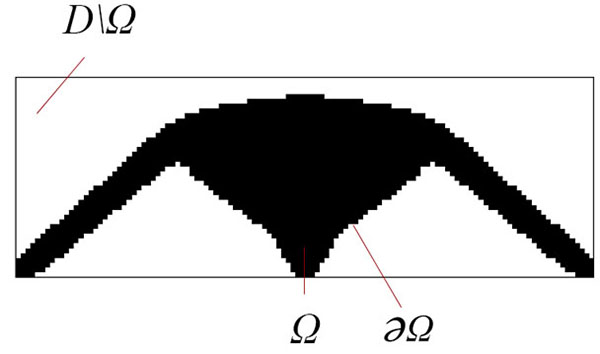
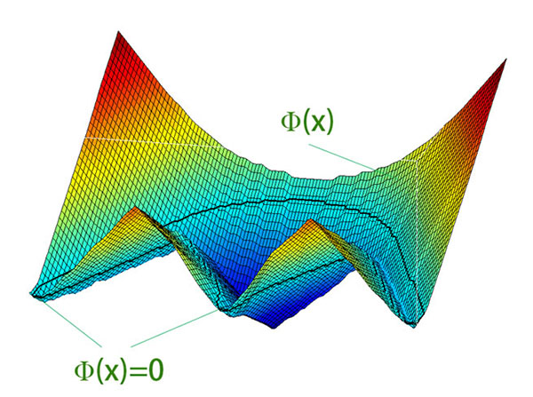
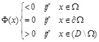
Fig. (2) illustrates that the two-dimensional boundary is defined by a zero level set of signed distance function, which occupies a three-dimensional space and is also a level set function. When the structure is a subset of some domain Ω, which lies in a bigger design domain D, the subsequent properties manifest themselves as follows:
 |
(1) |
in which
, as before, indicates the lower dimensional boundary, while Ф(x) denotes the level set function. In the optimization of structure, for simplicity, the level set of zero is usually used to indicate the boundary as
:
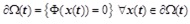 |
(2) |
Operating the preceding formula with differentiation gives the evolution formula for the level set function, which is defined with the subsequent Hamilton-Jacobi equation:
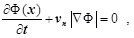 |
(3) |
where 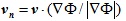 denotes normal component of velocity, while t denotes pseudo time.
When a function, which is described with less dimensions, is embedded into a function, which is described with more dimensions, there will be many favorable features [22]. Furthermore, representing the function described with more dimensions by a signed distance function facilitates the update process. Hence, the signed distance function is frequently used to represent the level set function at first. However, the degeneration of convergence properties emerges in the process of updating. Hence, the re-initialization techniques are required to regulate the level set function [23].
2.2. Structure Discretization
Prior to the optimization process, the structure is required to be discretized, after which the analytical sensitivities are calculated. With the aim of performing the finite element method on a non-conforming mesh, the relation between the level set function and the element density field pe, which is usually obtained by averaging the Heaviside function H, must be clearly defined:
 |
(4) |
in which Ωe is the material domain of e.
An approximate Heaviside function could be utilized to evaluate the element density, for example, a third order polynomial:
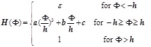 |
(5) |
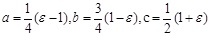 |
(6) |
where ε is the lower bound for the element densities and h denotes the bandwidth of the approximate Heaviside. When h → 0, it is transformed to the exact Heaviside and physically equals the volume fraction of material in each cell.
The density evaluated by the equation (5) is eligible to be directly applied to assess the stiffness, which is called the ersatz material approach. The stiffness element is evaluated by the following equation:
 |
(7) |
in which Ke denotes the elemental initial stiffness matrix, and u denotes displacement vector, while f denotes the external loading vector.
3. FORMULATION OF TOPOLOGY OPTIMIZATION PROBLEM
The objective of optimization is to reduce the weight of the structure and simultaneously find the optimal distribution of materials to maximize the structural stiffness. Therefore, structural compliance is an objective function. h(pe, u) Linear constraint is employed to demonstrate the linear attribute that the structure demonstrates, and nonlinear constraint g(pe) is used to demonstrate the volume fraction. The mathematical model of the topology optimization problem for continuum is defined by:
min
 |
(8) |
s.t.
 |
(9) |
 |
(10) |
 |
(11) |
where f is the external loading vector, Vmax and is the desired volume fraction. The element density
 varies between the lower bound and ε 1. The definition of ε is to evade singularity. The element density
is evaluated by equation (5).
varies between the lower bound and ε 1. The definition of ε is to evade singularity. The element density
is evaluated by equation (5).
4. SENSITIVITY ANALYSIS
4.1. Design Sensitivity
The evolvement of the level set function demands the message from the element sensitivities. If the moving boundary satisfies the traction-free boundary conditions, the subsequent formula could be used to define the design sensitivity of the compliance objective
 :
:
 |
(12) |
where
 is a coefficient, and it is a result of equation (7) for the avoidance of singularity, while u denotes the global displacement vector, and ue denotes the element displacement vector [24]. There is a significant difference between the formula of design sensitivity and the one employed by SIMP, as the densities defined in this work have been polarized while the avoidance of intermediate densities penalization is utilized. Straightforwardly, the design sensitivity with respect to volume constraint g(pe) is identical to that in [25]:
 |
(13) |
4.2. Topological Sensitivity
Let Ω be an open-bounded domain with a smooth boundary and set Ωe to be a new created domain, then:
 |
(14) |
in which the boundary can be expressed by:
 |
(15) |
 |
(16) |
where  denotes a sphere of radius ε with its center located at
 [26]. Hence, the new domain Ωe, which has the tiny hole
 , emerges. Usually a shape functional Ψ(Ωe), which has association with the topologically perturbed domain, accepts subsequent topological asymptotic expansion, which is expressed by:
 |
(17) |
in which Ψ(Ω) denotes a shape functional belonging to the unperturbed domain. Moreover, f(ε) denotes a function whose values are always positive, so that f(ε) → 0 when ε → 0. Then, function
 , which could be considered a first order correction of Ψ(Ω) to approximate, Ψ(Ωε) is used to express the topological sensitivity of ψ at
 . Rearranging equation (17) gives the following:
 |
(18) |
Limit passage ε → 0 of the preceding equation results in:
 |
(19) |
An inference about the topological optimization could be made by exploiting its geometrical interpretation. However, for the sake of making good use of topological sensitivity, an explicit numerical formula should be given. Topological sensitivity with respect to the two-dimensional objective function
, which aims to minimize the structural compliance and satisfies the traction-free boundary conditions on the newly created hole as regards a sphere with a radius of one as the model hole, is
 |
(20) |
where ueT(KTr)e ue is the finite element approximation to the product tr(σ)tr(ε*) in which σ and ε* separately denote the stress tensor and strain tensor [27]. In (17) λ and µ denote the Lamé parameters. The topological sensitivity with respect to volume constraint
 , which involves a sphere with a radius of one, is expressed by:
 |
(21) |
5. PROPOSED METHOD
For the compliance minimum problem, we propose an iterative algorithm incorporated with the level set method, design sensitivity, and topological sensitivity. We have implemented the algorithm with MATLAB. A level set function is established according to material boundary. As discussed, it is preferable to choose the signed distance function as a level set function for its virtue of simplicity shown in the function updating process. Then, the state equations are discretized on finite elements. For simplicity, bi-linear, four-node, square elements are used. After the process of finite element analysis, the global displacement vector u and elemental displacement vector ue will be returned, and the algorithm updates the level set function.
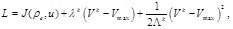
In the method proposed in this work, the sign of the design sensitivity is reversed and employed as the normal velocity vn for the boundary of the design. For the sake of avoidance of a local minimum, which consists of insufficient holes, topological sensitivity is incorporated into the proposed update scheme. A revised trapezoidal method is utilized to solve formula (3) of the update scheme so that a more accurate result is obtained. In comparison with the conventional level set method, the forward Euler method is always exploited. Based on formula (3) and the trapezoidal method, a revised and novel update scheme for the level set function is defined as follows:
 |
(22) |
in which  is a positive parameter, and Δt is a step size of time. To strike a balance between the influence of design sensitivity
and that of topological sensitivity must be well defined.
is a positive parameter, and Δt is a step size of time. To strike a balance between the influence of design sensitivity
and that of topological sensitivity must be well defined.
In addition, vn and η are the velocity terms that are defined by design sensitivity and topological sensitivity. To meet the volume constraint, both terms are defined by the Lagrangian design sensitivity and topological sensitivity:
 |
(23) |
where
 are parameters. They are updated at each iteration and described through the subsequent formula:
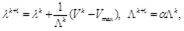 |
(24) |
where Vk is the volume of the current optimized result after k iterations. The coefficient
 should be a static coefficient. With Lagrangian and sensitivity outcomes, velocity vn, which is defined within element at k iterations, is expressed by:
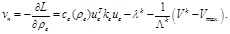 |
(25) |
The purpose of the velocity term η, which is chosen based on topological sensitivity, is to nucleate holes. However, nucleating a hole in a void region is pointless. Hence, g is defined by:
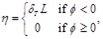 |
(26) |
in which δTL denotes the Lagrangian topological sensitivity that is expressed using:
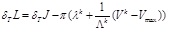 |
(27) |
Then, an iteration of optimization has finished. If the results converge, the whole optimization process will terminate. Otherwise, another iteration will begin.
The property of the level set function deteriorates as the update of the level set function proceeds. Thus, re-initialization of the set level set function back to the signed distance function is critical and required after a couple of steps. Without re-initialization, the optimized result would become unacceptable.
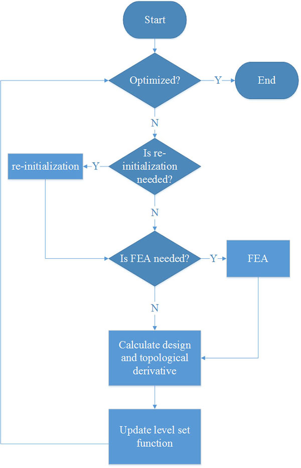
Finite element analysis is an extremely time-consuming process. Usually, the changes in the result of finite element analysis are trivial within a couple of update steps. With this observation, a parameter is set to decide how often finite element analysis is performed, and it results in a substantial decrease in the whole time of optimization. The flow chart of the proposed method is shown in Fig. (3).
6. NUMERICAL EXAMPLES
6.1. Design of a Cantilever
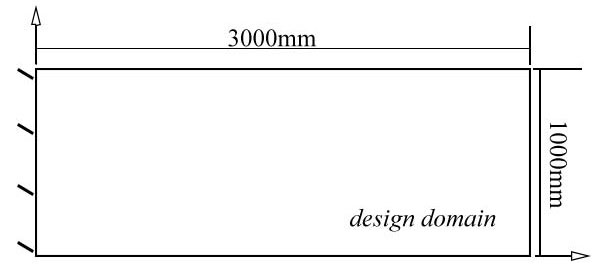
We consider the design of a cantilever that has a span of 3000 mm, height of 1000 mm, Young’s modulus = 100 GPa, and Poisson’s ratio v = 0.3. To simplify the problem, the material is deemed to be isotropic homogeneous. As depicted in Fig. (4), the design domain is subject to a loading of 100 N at the right center and is fixed on the left side. The volume fraction is 50%.
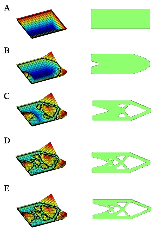
The whole design domain is discretized by a 60×20 finite element mesh. The original design domain, midway design results, final optimal results, and their corresponding level set function are shown in Fig. (5). Initially, the zero-contour of the level set function is set to be the whole design domain/material domain. The internal holes, which have to be set initially in conventional level set topology optimization, are not embedded. Then, the material domain shrinks due to the influence of the volume constraint. At the same time, the algorithm endeavors to nucleate internal holes spontaneously without initial assistance. After a couple of steps, the structure reaches its optimal result.
- Original design
- Midway design
- Midway design
- Midway design
- Final design
6.2. Design of Pylon
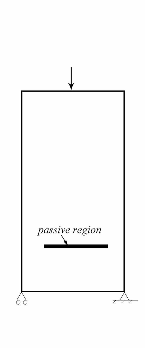
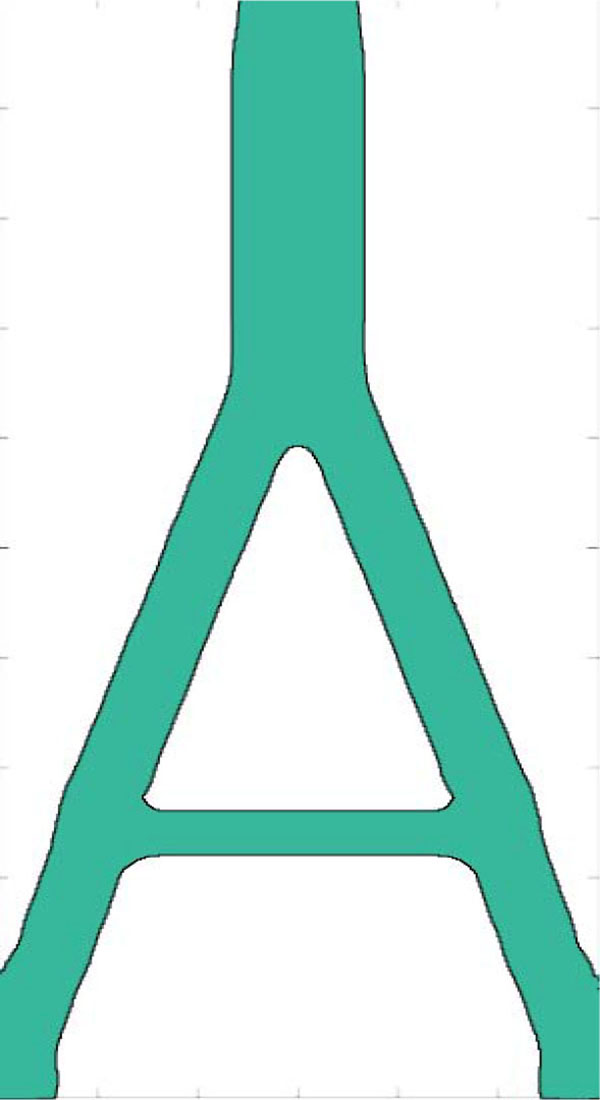
Then, the design for the inverted Y-shaped pylon is presented. The design domain is shown in Fig. (6) and is discretized in a 30×80 mesh. The passive region is composed of the elements that cannot be optimized. It can either be void or solid from the beginning to the end. At the center of the top side, a loading of 5000 kN is applied. A volume fraction of 40% is required. As shown in Fig. (7), the optimized result is similar to the real pylon. The Rama VIII bridge in the Thailand is shown in Fig. (8). The resemblance between the optimized result and the Rama VIII bridge is noticeable. They both are typical Y-shaped pylons.

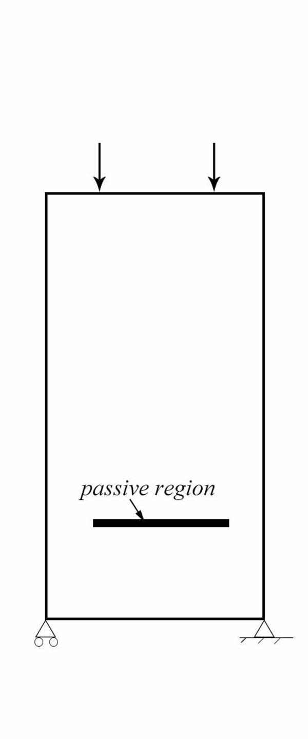
If there are two loadings of 2500 kN each at the upper side, the design result will be different. The design domain is shown in Fig. (9), and the volume fraction is 35%. The optimized result is depicted in Fig. (10).

CONCLUSION
For the sake of improving the accuracy of the conventional level set method and to assist engineers in design jobs with the level set method, a revised level set method for topology optimization is proposed using the trapezoidal method and topological sensitivity. Finite element analysis is utilized to discretize the structure. Based on result of the finite element analysis, the shape sensitivity and topological sensitivity are calculated to push and pull the boundary of material domain. In the conventional level set method, an initial guess of the number of internal holes is critical for its strong influence on the final optimized result. In the proposed method, the internal holes are nucleated spontaneously without an initial guess of the number of internal holes, and it manifests itself in the design of the cantilever, pylon and bridge tower. A flow chart of the algorithm implementing the proposed method is also provided. At the end, the design of the cantilever is presented to validate the proposed method. To demonstrate the utility, the proposed method is applied to the design of the inverted Y pylon and bridge tower. The optimized result for the inverted Y pylon design matches the practical designs very well.
The presented work only deals with the pylon and bridge tower design with simple loading case. The future work would extend the method to solve different optimization problems, such as dynamics issues. Also, the future work should address the issue of a structure that is meshed with irregular grids.
LIST OF ABBREVIATIONS
|
|
= a closed round sphere of radius ε |
| Bε | = an open round sphere of radius ε |
| ∂Be | = the boundary of
|
| ∂D | = the boundary of domain ∂D |
| ∂De | = the boundary of which has a round sphere of radius ε |
|
|
= the boundary of Ω |
| D | = the total computational domain for the optimization problem |
| ε | = a positive number that approximates 0 |
| ε* | = the strain tensor |
| f | = the external loading vector |
| g | = the non-linear constraint |
| H | = the Heaviside function |
| H | = an approximate Heaviside function |
| h | = the linear constraint |
| h | = the bandwidth of the approximate Heaviside |
| J | = the objective function |
| Ke | = the elemental stiffness matrix |
| K | = the global stiffness matrix |
| λ | = the Lamé's first parameter |
| µ | = the Lamé's second parameter |
 |
= the Lagrangian multipliers |
| η | = the velocity term defined by topological derivative |
| Ω | = the material domain |
| ψ | = a shape functional |
| Ф | = the level-set function for the domain |
| Ωe | = the open bounded domain with a round sphere of radius |
| ρe | = the element densities field |
| t | = time, used in the evolution equation for the level-set function |
| σ | = the stress tensor |
| δT* | = the topological derivative of |
| δTJ | = the topological derivative of objective function |
| δTg | = the topological derivative of volume constraint |
| δTL | = the topological derivative of Lagrangian |
| u | = the displacement vector |
| ue | = the elemental displacement vector |
| vn | = the normal component of velocity |
| v | = the design velocity field |
| vn | = the velocity term defined by shape derivative |
| x | = the coordinates of a point in the domain D |
|
|
= the coordinates of the center of
|
CONFLICT OF INTEREST
The authors confirm that this article content has no conflict of interest.
ACKNOWLEDGEMENTS
This work was supported by the National Natural Science Foundation of China under Grant No. 51175197.