All published articles of this journal are available on ScienceDirect.
Intelligent Computing Based Formulas to Predict the Settlement of Shallow Foundations on Cohesionless Soils
Abstract
Introduction:
Although it is a regular duty of geotechnical engineers to evaluate how much shallow foundation settles in the granular soil, there is no well-approved formula for this task. The intent of this research is to develop a formula that is adequately simple to be used in routine geotechnical engineering work but complete enough to address the behavior of granular soil associated with the settlement issue.
Methods:
Cone penetration test and foundation load test data were used to generate a formula that can predict the settlement. Genetic Programming (GP) based Symbolic Regression (GP-SR) and artificial neural networks were used to develop an optimized formula. Settlements were also calculated using the finite method and compared to the results of the developed formula.
Results and Conclusion:
Two formulas were developed using SR, and several models were developed using ANN. ANN model 1 has the highest R2 value (0.93) and the lowest MSE (0.16) among all developed ANN and GP-SR models. FEM settlements were almost double the measured ones in some instances.
1. INTRODUCTION
The foundation system carrying the loads of any structure can be either shallow or deep.
Shallow foundations are considered a feasible alternative because of their cost effectiveness, short construction time, and environmental friendliness. Typically, their design is dominated not by bearing capacity but by settlement. Because performance data is limited and predictions of settlements inflated, shallow foundations are frequently underutilized. Therefore, estimating the settlement is an important criterion to be considered in the design stage of shallow foundations.
Different methods, ranging from purely empirical to complex nonlinear finite elements, have been tried but has failed to produce accurate predictions of settlements [1]. Several researchers have studied the behavior of shallow foundations on cohesionless soils [2-12]. Most of them had examined how the results of calculated and field measured settlements of shallow foundations are compared to one another.
The principle factor in predicting settlement is the subsurface exploration data, specifically, its quality and quantity. Current in-situ tests notably the Cone Penetration Test, Standard Penetration (SPT), and Dilatometer Modulus (DMT) tests attempt to estimate the parameters of soils in the subsurface. Actually, in addition to its strong theoretical background, the CPT has several advantages: speed, economy, near continuousness, and repeatability. As Robertson [13] pointed out that these advantages have steadily advanced the CPT’s world-wide use and application. Furthermore, CPT data is useful in predicting settlement behaviors by applying the methods proposed by Schmertmann [14], Meyerhof [15], and DeBeer [16].
The goal of this study was to develop formulas to predict the settlement of shallow foundations on cohesionless soil using Genetic Programming (GP) based Symbolic Regression (GP-SR) and Artificial Neural Networks (ANNs). CPTs and foundation load tests data have been used, leading to a numerical formula that enables the accurate prediction of shallow-foundation settlement on granular soils. To develop and augment the formula, ANNs and GP-SR have been used with a database compiled from the results of 44 shallow foundation field load tests. There is a little application of GP-SR technique to predict the settlement of shallow foundation, using CPT and load tests, in the literature.
2. EXPERIMENTAL DATABASE
A database was compiled from the results of 44 square shallow foundation load tests (270 data point). All load tests were carried out post ground improvement work using Dynamic Compaction (DC) or Rapid Impact Compaction (RIC). Menard and Broise [17] were the first to expound the virtues of DC, and since then it has become a popular technique because it is simple, cost-effective, and reaches to significant depths. Moreover, although primarily testing granular fills and sandy materials, it works well with many other soil types and conditions, as well [18]. RIC applies low energy to compact sandy soil at shallow depths, thus filling the void between the DC and shallow compaction methods such as roller compaction [19].
All tests were performed according to the ASTM D1196/D1196M-12. Foundations were loaded to 150% of the design load. The applied testing load was produced by a hydraulic jack that had enough capacity for applying the maximum load needed and was equipped with a precisely calibrated gauge to point out the magnitude of the applied load. Reaction to the hydraulic jack was provided by a platform carrying concrete blocks. The platform was supported by an array of secondary steel beams and the main girder. Deflections (settlements) were measured about the fixed reference beams using dial gauges. Such deflections were monitored for each loading increment using four dial gauges. The average readings of the four dial gauges were taken as the settlement for the load increment. Before load testing, CPTs were performed at each location to estimate the soil parameters. The data collected at each test location included the width of the footing (B) in m, applied pressure (P) in kPa, settlement (S) in mm, and the average cone tip resistance (qc) in MPa for a 2B depth below the footing’s bottom.
Based on the work by Lunne et al. [20] and Robertson [13], the soil was classified at each test location according to CPT test results regarding Soil Behavior Type (SBT). The classifications were either clean sand-to-silty or gravelly sand-to-sand. It is to be noted that no cohesive soil was found in any of the test locations. The depth of the water table ranged from 0.5m to 1.75m below the bottom of the footing. This type of soil has a high permeability, and the pore water pressure is very low. Therefore, the groundwater table was not considered as an influencing factor in this research. The groundwater is important in soft, fine-grained soils where in-situ moisture takes a longer time to dissipate. Table 1 provides a summary of the collected data from each load test.
3. INTELLIGENT COMPUTING
Two intelligent computing techniques, Artificial Neural Networks and Symbolic Regression (SR), led to the development of a formula to predict the settlement of the shallow foundation. The input variables are cone tip resistance, applied pressure, and footing width. In order to evaluate the developed formula, a performance criterion was established. Three statistical measurements were utilized, the Mean Square Error (MSE), Mean Absolute Error (MAE), and the coefficient of determination (R2), with a goal of developing a formula with higher R2 value and the least MAE and MSE. The equations of these performance criteria are given below:
 |
(1) |
 |
(2) |
 |
(3) |
Where n is the total count of measurements, ei is the differences between actual (measured) values and predicted settlement values, Si is actual settlement values, and  is the average of the measured settlement values.
3.1. Symbolic Regression (SR)
Symbolic Regression can find mathematical formulas by minimizing errors. It is a function-finding technique for modeling numeric multivariate datasets. It is different from traditional regression in that it builds mathematical functions by searching the parameters and different forms of equations [21, 22]. It approaches a specific modeling problem by exploring nonlinear equation forms alongside their parameters, usually finding a mathematical function which can clarify the relationship between dependent and independent variables [22, 23]. SR is an application of genetic programming, and, because it requires no special knowledge to create free-form mathematical models from collected data, it is an appealing option to the standard regression method. A Genetic Programming GP-based Symbolic Regression (GP-SR) software, Eureqa [24], was utilized in this research to develop a formula that can predict the settlements.
| Collected Variable | Mean | Standard Deviation | Min. | Max. | Range |
|---|---|---|---|---|---|
| qc ( MPa) | 11.73 | 1.69 | 8.57 | 14.5 | 5.93 |
| B (m) | 2.12 | 0.24 | 1.5 | 3.0 | 1.5 |
| P (kPa) | 141.21 | 83.03 | 18.75 | 375 | 356.25 |
| S (mm) | 4.08 | 2.21 | 0.24 | 11.79 | 11.55 |
| No. | Formula | R2 | MSE | MAE |
|---|---|---|---|---|
| 1 |  |
0.84 | 1.62 | 0.44 |
| 2 | 18.3+0.016P+0.0352Bqc2-2.59qc | 0.78 | 2.13 | 0.62 |
A set of input variables (P, qc, B), with its experimental settlement results (S), was used for the GP-SR. Mathematical operators were defined for use in the developed formula. Various combinations of operators and variables were then generated via a genetic algorithm in order to develop a symbolic equation that reflects an appropriate approximation. Developed equations were subsequently rated according to complexity and fit, based on the R2, MSE, and MAE. The results of the symbolic regression analysis are shown in Table 2). Two equations were developed to predict the settlement (S) using P, qc and B. R2. Values for those models were 0.84 and 0.78. MSE values were 1.62 and 2.13, while the MAE values were 0.44 and 0.62.
3.2. Artificial Neural Networks (ANNs)
Many previous investigations into geotechnical engineering have used artificial intelligence and ANN [25-31].
Shi et al. [32] offered a study of neural networks for predicting settlements of tunnels. Using SPT data, Shahin et al. [33] presented an artificial neural network model designed to predict the settlement of shallow foundations on cohesionless soils. Nejad et al. [34] developed an ANN model to predict pile settlement based on standard penetration testing. The ANN developed by Tatari et al. [35] assesses the condition of culverts based on inventory data presented by Masada et al. [36, 37]. Tarawneh [38] and Tarawneh and Imam [39] developed ANN models using dynamic load testing that can predict pile setup for three pile types (pipe, concrete, and H-pile). Tarawneh and Nazzal [40] employed ANN to optimize the prediction of subgrade resilient modulus design input from falling weight deflectometer test results.
The functioned approximation techniques of ANNs can be used in a nonlinear, complex contact nature between input(s) and output(s). ANN is considered a soft computing method that imitates how the human brain processes information-transfer [41]. Among the different types of ANNs, the multilayer feed forward ANN is the most frequently used. It consists of input, hidden, and output layers which are connected by different connection weights. For the optimum outcome, ANNs should be trained through learning algorithms, such as the most widely used back-propagation [42]. The basis for that algorithm is a gradient descendent optimization procedure that minimizes the MSE (average mean squared error) between the predicted and desired values/outputs.
In this research, the ANN model input variables are applied pressure (P), CPT tip resistance (qc), and width of square footing (B). The ANN model output is Settlement (S). The data was divided into three sets: training, cross-validation, and testing. Seventy percent of the data points were selected for training, 15% for cross-validation, and 15% for testing the network. The training data points were used to train the network and compute the weights of the inputs. The test data points established the performance level of the selected ANN model. Cross validation measured test-set error during the period in which the network was going through the training set [30].
It is essential that the data used for training, cross-validation, and testing characterize the same population and its statistical properties. Constructing the best model possible necessitates a training set that includes all of the patterns that the data contains. Likewise, the test set determines when to stop training; therefore, it should be representative of the training set and should contain all patterns existing in the available data [43]. To achieve this, numerous random combinations of the training, cross validation, and testing sets were engaged until a statistically reliable data set was obtained.
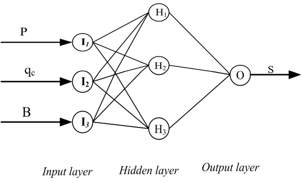
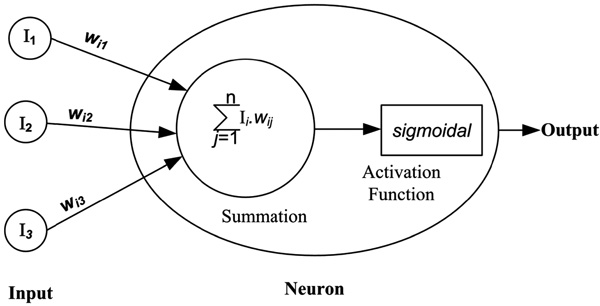
Numerous network structures, with different numbers of hidden layers and nodes in the hidden layer, were trained and tested to find the model with the best performing network architecture. Because it has been shown that a network with one hidden layer can approximate any continuous function [44], in this research one hidden layer was used. Typically, the structure of ANNs includes processing elements (PEs), or nodes, that are arranged in three layers input, output, and hidden (Fig. 1). Every PE in each layer is joined, whether totally or partly, to other PEs by weighted connections. The input from each PE in the previous layer (Ii) is multiplied by an adjustable connection weight (wij). The weighted input signals are summed at each PE, at which point a bias (Ɵi) is added. This combined input (Ii) is then passed through a sigmoidal transfer function or other nonlinear transfer function to produce the PE’s output (yi), which provides the input to the PEs in the next layer. Equations 4 and 5 show this process, and Figs. (1 and 2) describe it.
 |
(4) |
 |
(5) |
To develop optimal network geometry, ANNs with a single hidden layer and a different number of nodes in the hidden layer were trained with sigmoid (Sig.) and hyperbolic tangent (tanh) transfer functions for the hidden and output layers. Combinations of the number of elements in the hidden layer and types of the transfer function that yielded the most accurate predictions of settlement (S) are shown in Table 3.
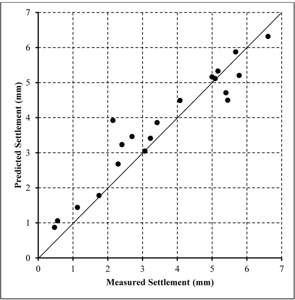
Table 3 shows that model 1 has the greatest R2 value and the least MSE and MAE values for the testing data set. The plot of the measured and predicted settlements for the model’s testing data set is shown in Fig. (3). This model is the best performer among the developed ANNs and SR. The mathematical expression of the ANN algorithm is presented below:
4. VERIFICATION OF THE SELECTED ANN MODEL
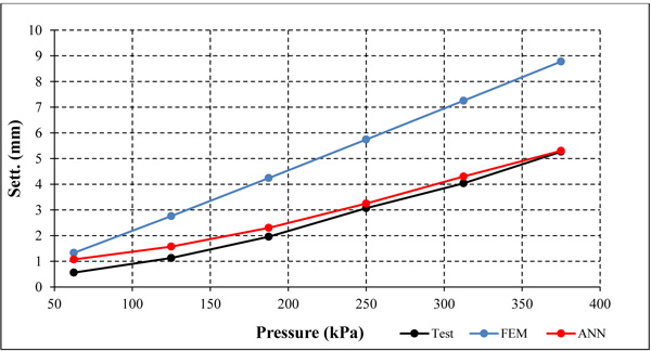
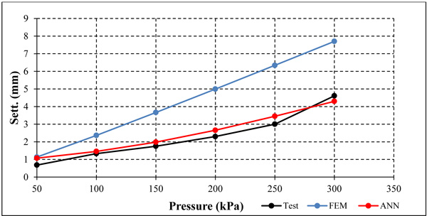
A separate shallow foundation three load test was used to verify the selected ANN model. Settlements were estimated using the Finite Element Method (FEM) and compared with the outcomes from the ANN model and the measured settlements of those load tests.
The load test was performed in agreement with the ASTM D1196/D1196M-12. The tests were carried out using 2.5m-wide footing on a sandy soil. Table 4 shows the average tip resistance (qc) within 5m below the bottom of the footing, pressure, and measured settlements.
4.1. Settlement Estimation using Finite Element Method (FEM)
Settlements were estimated using FEM. The conventional, Mohr-Coulomb soil model was used in the analysis process. This elastic perfectly plastic model relies on a combination between Hooke’s law and the Coulomb’s failure criterion. That is, it has five input parameters, including Young’s modulus and Poisson’s ratio for soil elasticity, angle of friction and cohesion for soil plasticity, and the angle of dilatancy. Soil input parameters were estimated based on CPT data as presented by Robertson [13]. Soil parameters are shown in Table 5. Midas Soil Works FEM software was utilized to perform the analyses.
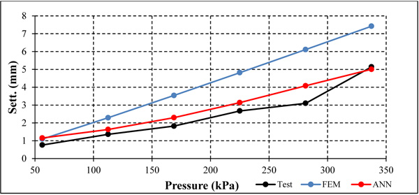
A comparison was made between the results of the finite element analysis and the measured settlements and predicted values by ANN model as shown in Figs. (4 to 6). Those figures clearly demonstrate the superior performance of the developed ANN model over the FEM. Settlements estimated by ANN are comparable to those measured from load tests. In all tests, FEM over-predicted the settlements, giving conservative predictions. FEM settlements are almost double the measured ones in some cases, as shown in those figures. It should be noted that ANN is over-predicting the settlements by a value of less than one millimetre and half millimetre for load test-1 and 2, respectively.
| Model No. | Input Nodes | Hidden Layer-1 | Output Layer | Testing Data | ||||
|---|---|---|---|---|---|---|---|---|
| Processing Elements | Transfer Function | Processing Elements | Transfer Function | MSE | MAE | R2 | ||
| 1 | 3 | 3 | Sig. | 1 | Sig. | 0.16 | 0.2 | 0.93 |
| 2 | 3 | 3 | tanh | 1 | tanh | 0.21 | 0.27 | 0.87 |
| 3 | 3 | 4 | tanh | 1 | tanh | 0.26 | 0.33 | 0.82 |
| 4 | 3 | 5 | Sig. | 1 | Sig. | 0.29 | 0.36 | 0.79 |
| 5 | 3 | 6 | tanh | 1 | tanh | 0.33 | 0.41 | 0.79 |
 |
(6) |
Where A1, A2, and A3 can be calculated using the equations below:
 |
(7) |
 |
(8) |
 |
(9) |
| Load Test No. | B (m) | qc ( average of 5m below footing) | Pressure (kPa) | Measured Settlement (mm) |
|---|---|---|---|---|
| 1 | 2.5 | 10.8 | 56.25 | 0.76 |
| 112.5 | 1.36 | |||
| 168.75 | 1.82 | |||
| 225 | 2.67 | |||
| 281.25 | 3.1 | |||
| 337.5 | 5.14 | |||
| 2 | 2.5 | 12.84 | 62.5 | 0.56 |
| 125 | 1.13 | |||
| 187.5 | 1.96 | |||
| 250 | 3.07 | |||
| 312.5 | 4.04 | |||
| 375 | 5.27 | |||
| 3 | 2.5 | 11.46 | 50 | 0.68 |
| 100 | 1.33 | |||
| 150 | 1.75 | |||
| 200 | 2.30 | |||
| 250 | 3.0 | |||
| 300 | 4.61 |
| Soil Parameter | Values Range |
|---|---|
| Soil cohesion, C (kN/m2) | None cohesive soil ( C=0 ) |
| Soil friction angle, ϕo | 33- 40 |
| Angle of dilatancy ( ψο) | 3-10 |
| Young’s modulus ( kN/m2) | 2.5qc |
| Poisson’s ratio (μ) | 0.3 |
SUMMARY AND CONCLUSION
This paper has presented the results of a study that was conducted to evaluate the use of SR and ANNs to develop a formula that can accurately estimate settlement of shallow foundations on cohesionless soils. From 44 square shallow foundation load tests, post ground improvement, a database was compiled. At all test locations, soil was classified as either clean sand-to-silty sand or gravelly sand-to-sand. There was no cohesive soil present in any of the test locations. The depth of the water table was 0.5m to 1.75m below the bottom of the footing.
ANN and SR were employed to develop a formula that can reliably predict the settlement. The input variables were cone tip resistance, applied pressure, and footing width. To evaluate the developed formula, a performance criterion was established using MSE, MAE, and R2. The goal was to develop a formula with highest R2 value and least MAE and MSE. Two formulas were developed using SR (Table 2), and several models were developed using ANN. As shown in Table 3, ANN model 1 has the highest R2 value (0.93) and the lowest MSE (0.16) and MAE (0.2) among all developed ANN and SR models.
A separate shallow foundation three load tests verified the selected ANN model. Further, settlements were estimated using FEM and compared with the results of the selected ANN model and the measured settlements of those load tests. In all tests, FEM over predicted the settlements, giving conservative predictions. FEM settlements were almost double the measured ones in some instances.
It can be concluded that the ANN model is a satisfactory predictor of the settlements of shallow foundation on cohesionless soils. A benefit of ANNs is that, once the formula is trained, it can be utilized as a quick method for settlement estimation. Conversely, the main disadvantage of ANNs is insufficient theory to foster their development and their limited ability to explain the method by which they analyze the available data to achieve a solution. It should be noted that the ANN modeling hinges on experimental data and is applicable for use in an interpolative sense. As an empirical formula, the scope of its applicability is controlled by the data used to build and calibrate the model. To update the model and increase its accuracy, it is important to include additional data to enable the model to be re-trained.
Despite the above-mentioned shortcomings, the results of this research point out that ANNs have several significant powerful and practical benefits that make them a valuable tool in predicting the settlement of shallow foundations on cohesionless soils. It should be noted that the developed formulas can only be used for similar type of soils.
CONSENT FOR PUBLICATION
Not applicable.
CONFLICT OF INTEREST
The authors declare no conflict of interest, financial or otherwise.
ACKNOWLEDGEMENTS
The authors would like to acknowledge the collaboration and assistance of both Menard Vibro Middle East and RIC Middle East in Dubai, UAE.

