All published articles of this journal are available on ScienceDirect.

Simulation of Pressure Head and Chlorine Decay in a Water Distribution Network: A Case Study
Abstract
Background:
The main issue in the operation of water distribution systems arises from the pressure deficiency resulting from events such as loss from leaks and bursts and loss of hydraulic capacity due to deterioration of aging water pipes. Such conditions affect the hydraulic performance of the system and the quality of water.
Objective
This paper investigates the hydraulic and water quality behavior of a selected water distribution network in Makkah city using the EPANET software.
Methodology:
The system was simulated under different hydraulic conditions including a loss of hydraulic capacity with pipe age and the presence of 30% leakage in the network over varying time conditions by employing extended period simulation models.
Results and Conclusion:
The results show that increasing pipe roughness with pipe age resulted in significantly low-pressure heads at the end of the network-particularly during peak demand hours. It also resulted in an increase in the rate of chlorine decay. Leakage in the network significantly affects the pressure head, resulting in pressure deficiency at some points in the network to below the minimum requirement during regular operation. The highest leakage rate occurs at periods of low demand where the pressure head in the network is high.
1. INTRODUCTION
Water Distribution Networks (WDNs) provide adequate water requirements for various usages, including domestic, commercial, and industrial purposes. They must meet demands at each node at all times and at a sufficient pressure head. However, the main challenge currently in the operation of WDNs comes from pressure deficiencies resulting from events such as loss from leaks and bursts, as well as loss of hydraulic capacity because of deterioration of aging water pipes. These conditions affect the hydraulic performance of the system and water quality. Thus, it is necessary to consider the effect of such conditions on the hydraulic and water quality behavior in WDNs.
1.1. Leaks in Water Distribution Networks
Leaks in Water Distribution Systems (WDSs) are a well-documented issue that affects both customers and suppliers. According to the World Bank [1], ‘real losses’ from these systems globally amount to more than 32 billion m3 of treated water annually-an estimated global average of 20%. Even more concerningly, in some low-income countries, this loss represents 40-50% of water supplied. In Saudi Arabia, the rate of leakage from water systems is estimated to be around 30% of water supplied [2].
Existing models attempt to model leaks from WDSs using the orifice flow equation (Eq. 1), which suggests that leakage is proportional to the square root of the pressure head in the pipe.
 |
(1) |
Here, q is the rate of flow, Cd is the discharge coefficient, Ao is the orifice area (area of the leak), g is gravitational acceleration, and h is the pressure head. In practice, a more general leakage Eq (2) is used [3].
 |
(2) |
where C and N1 are the leakage coefficient and leakage exponent, respectively.
However, field and experimental studies [4, 5] show that leakage rates could be much more sensitive to the pipe pressure head than suggested by the orifice flow equation (i.e., leakage exponent with theoretical orifice value of 0.5). Leakages differ with pressure in response to a value for the power exponent varying between 0.36 and 2.95 [4], which indicates that leakages in WDSs are strongly affected by pressure.
1.2. Loss of Hydraulic Capacity with Pipe Age
A number of research studies have considered the impacts of aging pipes on water transmission [6, 7]. Colebrook and White examined the issue of pipe roughness changing with time and found that build-up of material on the inside wall of the pipe increased pipe roughness and reduced pipe diameter. The effect of aging infrastructure is demonstrated in the Hazen-Williams coefficients CHW (Table 1). These data indicate that the carrying capacity of a 30-year old pipe is approximately 60% of the capacity of a new pipe.
| Age | Value of CHW |
|---|---|
| New | 130 |
| 5 years | 120 |
| 10 years | 107-113 |
| 20 years | 90-100 |
| 30 years | 75-90 |
1.3. Water Quality Deterioration in Distribution Systems
Deterioration of water quality in distribution networks has been studied by many researchers [9-15, 16, 17]. Seyoum and Tanyimboh [9] indicated that pressure deficiency in WDNs is the main determinant of the deterioration of water quality. Deficiency in pressure leads to low flow velocities, resulting in long water travel and detention time, which in turn, contribute to loss of disinflation residual. Nkontcheu et al. [10] conducted a study concerning pesticides as water pollutants and concluded that products comprised of imidacloprid and lambda-cyhalothrin should be handled carefully and away from water bodies. In a case study, Khudair et al. [12] predicted groundwater quality for drinking purposes based on a Water Quality Index (WQI). They used an artificial neural network model, which was found to provide high prediction efficiency; however, other important parameters, such as chloride and pH, affected the model prediction. Mohammed and Abdulrazzaq [13] developed another WQI method to evaluate the quality of drinking water based on eight water quality parameters. The suggested classifications in this method are excellent, good, acceptable, poor, and very poor. Nodoushan [14] presented successful applications of ANN and Bayesian networks (BN) to predict water quality parameters, such as salinity, temperature, and DO, on a monthly scale. The outputs showed that BN models outperform ANN models.
Clark et al. conducted laboratory tests to improve mathematical models of contaminant and chlorine propagation in distribution systems [15]. They found that the chlorine demand of pipes was significantly higher than the chlorine decay in the bulk water phase. This finding was attributed to the existence of biofilm on their inner surfaces. Jami [16] studied hydraulic and water quality behavior for two different pipe materials-mild steel (MS) and ultra-high-molecular-weight poly-ethylene (UHMWPE)-and concluded that the UHMWPE pipes performed better than MS pipes in terms of maintaining water quality in the system, as the MS pipes consumed nearly twice the amount of chlorine as the UHMWPE pipes.
Bensoltane et al. [17] proposed a method for the enhancement of residual chlorine concentration in a water supply network, combining numerical simulation using EPANET software and field measurements. The model was then calibrated, and the simulation tool used to predict chlorine decay behavior. The appropriate doses of chlorine could then be injected to enhance concentration throughout the network.
Ozdemir and Ucak [18] proposed a model for assessing chlorine decay in WDNs that used a simplified expression of a two-dimensional chlorine transport and decay formula with a single pipe that incorporated the bulk-flow reaction, radial diffusion, and subsequent pipe wall reaction of chlorine. The model outcomes were compared with observed chlorine measurements and EPANET outputs and showed good agreement.
Thus, researchers have made substantial efforts to study the hydraulic behavior of water pipe networks from different viewpoints. However, each water distribution system has its own characteristics. Further, because field measurements are often difficult, time-consuming, and costly, it is necessary to use computer software to explore the hydraulic and water quality behavior of a network.
Recently, the utilization of computer software has increased in line with the need for improvements in the operational efficiency of WDSs. Computer software can be used for a number of applications, including operational applications, optimization, and water quality analysis [19-21].
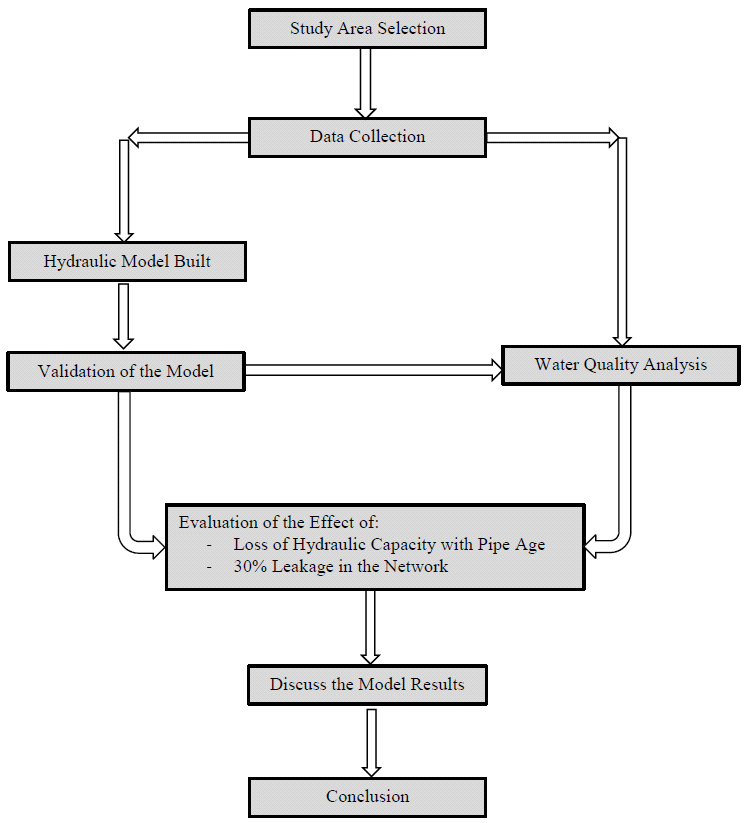
This paper investigates the hydraulic and water quality behavior of a selected water distribution network in Makkah city using EPANET computer software. It models and simulates the pressure head and chlorine concentration in the network under different conditions. Fig. (1) describes the schematic diagram of the research methodology. The results provide implications for designers and operators of WDSs.
2. METHODS
2.1. Hydraulic Model
Various computer models are now available and used in the water industry to forecast and evaluate the hydraulic performance in WDSs. The hydraulic analysis determines the pressure head, flow rate, velocity, and head loss in each element of the system. EPANET is one of the most frequently used WDN models [22]; it has been broadly utilized in research and industry and constitutes the basis for several commercial WDS modeling packages, including H2OMAP, PipelineNet, and WaterCAd [22].
The EPANET software was developed by the U.S. Environmental Protection Agency and can be used to simulate steady-state conditions and extended period simulations of hydraulic and water quality behavior in WDNs [23]. EPANET tracks the water flow in each pipe, the head at each node, and the height of water in each tank. It also can be used to simulate the concentration of a chemical species, water age, and source tracing throughout the network during a simulation period.
The EPANET water quality model is dynamic and incorporates relevant stage processes such as transport (i.e., advection) and various conversion processes such as chlorine decay [9]. As reported by Rossman [23], EPANET follows the fate of discrete parcels of water as they flow in pipes and mix together at nodes between fixed-length time steps. For each step, the mixture of each segment reacts, and a cumulative account is kept of the total mass and flow volume entering each junction; the locations of the segments are then updated [23]. The concentration of chlorine leaving the node is basically the flow-weighted sum of the concentrations from inflowing pipes and outside sources.
2.2. Area Under Study
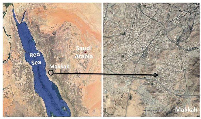
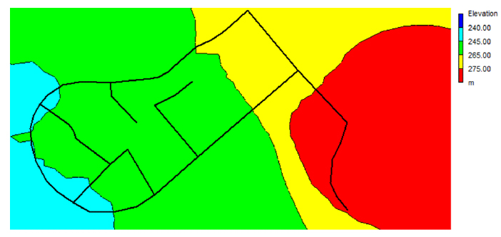
The area selected for this study is situated in Makkah city, Saudi Arabia. It is a residential area with an estimated population of 33,984, measuring 2000 m x 1000 m and located at 21º21’58”N, 39º50’21”E (Fig. 2). The elevation of the area ranges from 230–344 m above mean sea level (see the general elevation contour map produced by EPANET in Fig. (3).
2.2.1. Water Supply Network Model
The network is medium-sized and similar in nature to many other networks in the city of Makkah. The main source of water is a large water tank feeding the network. The tank is circular and 30 m in diameter with a water depth of 20 m. It is situated on the highest elevated spot (332 m), and the network is fed by gravity. The water tank draws desalinated water from Shoaiba desalination plant via a pumping station.
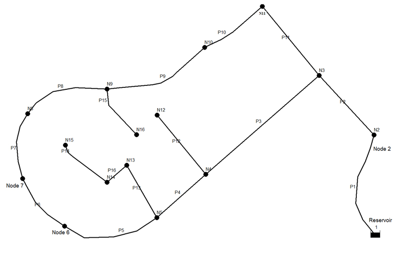
The simulation network layout is displayed in Fig. (4), including ID labels for the various components (i.e., nodes, pipes, and reservoir). The average base demand and elevation of each node in the network is shown in Table 2. The total length of pipelines is approximately 8.3 km, with different pipe diameters ranging between 80 mm and 300 mm. All pipes are made of ductile iron (Table 3).
For new ductile iron pipes, the Hazen-William roughness coefficient CHW is 145 [25]. However, it is well documented that pipe roughness changes over time. Due to the incrustation and tuberculation of corrosion products on the pipe walls, the roughness of pipes tends to increase. This increase in roughness results in a lower Hazen-Williams CHW factor, which leads to a higher frictional head loss in the pipe flow. The head loss in each pipe is calculated using the same roughness coefficient in the Hazen-William equation (CHW of 145 was assumed to start the analysis). To evaluate the effect of pipe roughness changes over time, further simulations were run with the same pipe network but roughness coefficients of 140, 135 and 130, representing CHW roughness coefficients after 20, 30, and 60 years of service, respectively [25].
2.2.2. Daily Demand Curves
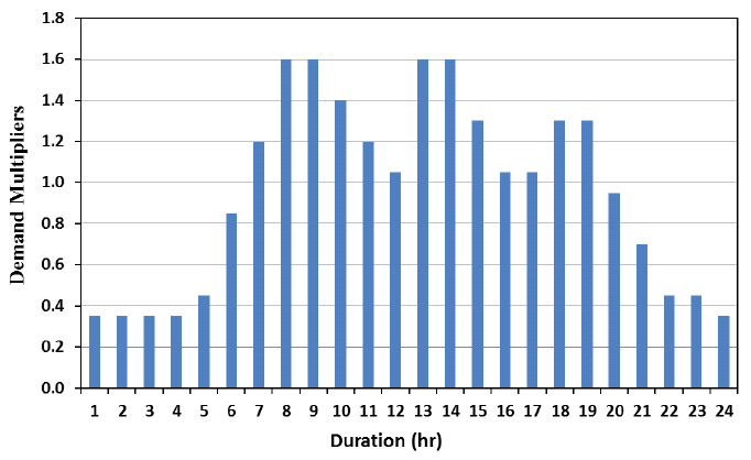
Water demand is highly variable throughout the day. This study has therefore adopted a daily curve that periodically varies throughout the day to render the simulation more realistic when analyzing an extended period of simulation. The standard daily demand curve for medium-sized cities developed by AWWA [26] was used for simulation in this study (Fig. 5). The curve shows how the water consumption rate changes over the day (24 hours) and provides the highest demand factors as multipliers that can be applied to the average base demand at a specific time. The same approach has been adopted in other studies [7].
| Node ID | Elevation (m) | Base Demand (l/s) | Node ID | Elevation (m) | Base Demand (l/s) |
|---|---|---|---|---|---|
| Node 2 | 281 | 0 | Node 10 | 265 | 3.43 |
| Node 3 | 274 | 0 | Node 11 | 267 | 0 |
| Node 4 | 247 | 0 | Node 12 | 254 | 14.18 |
| Node 5 | 247 | 0 | Node 13 | 252 | 10.81 |
| Node 6 | 241 | 4.18 | Node 14 | 249 | 3.75 |
| Node 7 | 244 | 6.25 | Node 15 | 263 | 8.12 |
| Node 8 | 243 | 3.93 | Node 16 | 254 | 3.75 |
| Node 9 | 249 | 3 | Resvr 1 | 332 | - |
| Pipe Number | Length (m) | Diameter (mm) | Pipe Number | Length (m) | Diameter (mm) |
|---|---|---|---|---|---|
| P1 | 709.71 | 300 | P9 | 724.6 | 120 |
| P2 | 527.45 | 300 | P10 | 465.3 | 150 |
| P3 | 981.22 | 250 | P11 | 583.02 | 150 |
| P4 | 426.45 | 150 | P12 | 499.36 | 150 |
| P5 | 655.1 | 100 | P13 | 393.35 | 150 |
| P6 | 422.24 | 80 | P14 | 371.32 | 100 |
| P7 | 451.59 | 80 | P15 | 369.77 | 80 |
| P8 | 577.66 | 100 | P16 | 169.69 | 150 |
2.2.3. Chlorine Reaction Coefficients
EPANET’s water quality model simulates chlorine decay considering the phenomena of chlorine reaction with chemical species in bulk fluid (kb) and pipe walls (kw).
The coefficients of the decay rate (both the bulk decay and the wall decay) for chlorine can change greatly, with the bulk decay coefficient changing with water quality and the wall decay coefficient changing with pipe material and condition [27]. Therefore, the pipe wall coefficient (kw) can be linked to the age and material of the pipe. The values for bulk fluid (kb) and pipe walls (kw) in this study were assumed to be -0.1008 / day and -0.20 m / day, respectively, as reported in other studies [7]. According to the World Health Organization (WHO) [28], the minimum safe concentration of chlorine in a water network is 0.2-0.5 mg/L.
3. RESULTS AND DISCUSSION
Initial runs using the simulation software (EPANET) revealed that the hydraulic behavior of the network was generally good. All hydraulic parameters including velocities in the pipes, pressures at the nodes, and head losses were checked throughout the network and determined to be under control. After validation of the network, the hydraulic performance was evaluated under different hydraulic conditions, including a loss of hydraulic capacity with pipe age and the presence of 30% leakage in the network over varying time conditions by employing extended period simulation models.
3.1. Effect of Pipe Age
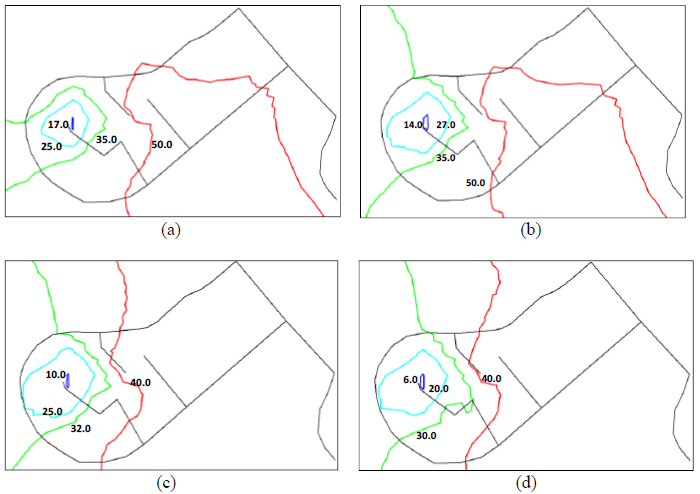
The effect of increasing pipe roughness with pipe age on the hydraulic performance of the network was analyzed at peak hour (i.e., 7 am) and shown in Fig. (6). It can be seen that the pressure head in the network ranges from 17–50 m for a Hazen-William roughness coefficient (CHW) of 145 (Fig. 6a); when the roughness coefficient is 130, the variation in the pressure head ranges between 6 and 40 m (Fig. 6d). This clearly shows a significant drop in the pressure head at some parts of the network, which in turn, requires further increases in energy to pump water to consumers. Further, with an increasing population and increasing water demand per capita, the likelihood of low water pressure in water systems is certain to increase.
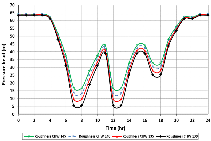
Fig. (7) shows the effect of pipe roughness changes with pipe age on the pressure head at node 15 over a day (24 hours). Pressure head is also affected by water demand, which is highly variable throughout the day. It can be seen that increasing pipe roughness (i.e., a lower Hazen-Williams CHW factor) resulted in significantly low-pressure heads at peak demand (i.e., 7 am and 12 pm). The pressure heads dropped to about 5.5 m when the roughness coefficient was 130-below the acceptable minimum pressure of 14 m required to deliver a minimum flow and overcome head losses in the client’s service pipe, meter, and house piping in the second floor of the house [29].
3.2. Chlorine Concentration in the Network
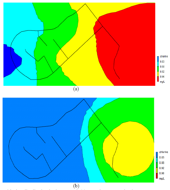
Fig. (8) shows the chlorine concentration in the network at initial run generated using EPANET at the peak and lowest demand hours of the day. The contour plots show that the concentration of chlorine in all parts of the network remains above the 0.2 mg/L recommended by the WHO [28]. The contour plots (Fig. 8) show that the concentration of chlorine in the network is higher during the peak periods of demand, and decreases during the lowest demand periods. One reason for this is that the water velocity in the network is higher and the conveyance of chlorine is more effective during peak water demand periods. Likewise, water velocity decreases at low demand periods; thus, the conveyance of chlorine throughout the network slows down, resulting in lower concentrations.
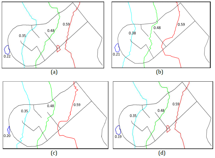
3.3. Effect of Roughness Coefficient on Chlorine Concentration
As discussed above, the wall decay coefficient changes depending on pipe material and condition. Therefore, the wall reaction coefficient can be related to pipe age and material. Fig. (9) shows this effect via contour plots of chlorine concentration in the network for different roughness coefficients. There is some evidence to support the view that the same processes that increase the roughness of a pipe with age will also lead to increased reactivity of its wall with some chemical species, such as chlorine and other disinfectants [30]. Fig. (9) shows that the chlorine decay rate tends to increase with increasing pipe roughness (i.e., lower CHW values). This finding is consistent with the observations of Clark and Rossman [31] and Mohamed and Abozeid [7]. Clark and Rossman [31] showed that chlorine residue in a water distribution network depends on a number of factors, including flow velocity, residence time, the diameter of the pipe, as well as bulk and wall decay rates.
3.4. Effect of Leaks in the Network
Leaks in WDSs are well-documented; an estimated 30% of treated water is lost from the network in Saudi Arabia. Assuming this percentage of leakage from a total network water inflow of 98.3 L/s implies a leakage rate of 29.44 L/s. Modeling leakage in a network can be obtained by adopting the approach of Cobacho et al. [32] to include leakage in network models. The leakage rate (i.e., 29.44 L/s) was added as a further demand at each node (i.e., 1.96 L/s). Considering that the pressure head in the network is about 40 m on average-and assuming a pressure exponent of 1.15-the emitter coefficient C in Eq. 2 has a value of 29.44 / (40)^1.15 = 0.42.
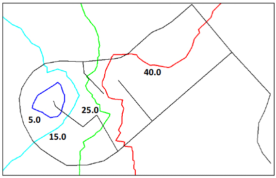
Fig. (10) demonstrates the effect of leakage on the pressure head distribution in the network. It can be seen that the pressure head drops from a range of 17-50 m in the normal operation case (Fig. 6a) to a range of 5-40 m in the case of 30% leakage in the network.
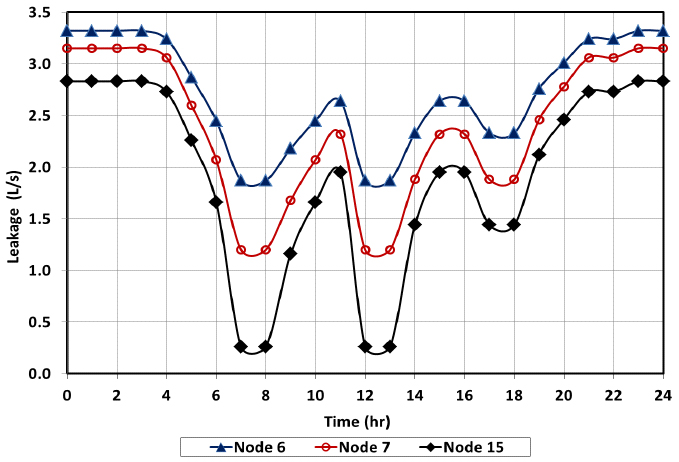
Fig. (11) shows the leakage rate over the day at three different nodes in the network (nodes 6, 7 and 15). Generally, it can be seen that the leakage rate is higher in periods of low demand (late evening to early morning). During this period, the pressure head in the network is high because of the low consummation rate. The highest leakage rate found is 3.32 L/s at node 6, which has the lowest elevation. Leakage wastes water and revenue and leads to inefficient distribution of energy through the network (i.e., wasted energy to pump water).
CONCLUSION
The approach of this research study was to model and simulate the hydraulic and water quality behavior of a selected water distribution network in Makkah city. EPANET was used for modeling and simulating the pressure head and chlorine decay in the network under different hydraulic conditions.
Based on this study, the following conclusions can be drawn:
- Increasing pipe roughness with pipe age resulted in significantly lower pressure heads at the end of the network during peak hours. With population increases and increasing water demand per capita, the likelihood of low water pressure in water systems will be intensified.
- Leakage in the network wastes water and energy. The presence of a 30% leakage rate resulted in a pressure deficiency at some points in the network. The leakage rate increases in periods of low demand, when the pressure head in the network is high.
- Distribution of chlorine concentration in the network is affected by hydraulic conditions. Increasing pipe roughness due to aging pipes resulted in an increase in the chlorine decay rate. The concentration of chlorine in the network is higher during the peak demand periods and declines during the lowest demand periods.
- Pressure deficiency in some parts of the network leads to deterioration of water quality in the network.
The results of the study are important to designers and operators of WDSs.
LIST OF ABBREVIATIONS
| ANN | = Artificial Neural Network |
| AWWA | = American Water Works Association |
| Ao | = Orifice Area (Area of the Leak) |
| BN | = Bayesian Networks |
| C | = Leakage / Emitter Coefficient |
| Cd | = Discharge Coefficient |
| CHW | = Hazen-Williams Coefficient |
| DO | = Dissolved Oxygen |
| g | = Gravitational Acceleration |
| h | = Pressure Head |
| kb | = Bulk Fluid Coefficient |
| kw | = Pipe Walls Coefficient |
| N1 | = Leakage Exponent |
| MS | = Mild Steel Pipe |
| q | = Rate of Flow |
| UHMWPE | = Ultra-High-Molecular-Weight Poly-Ethylene Pipe |
| WDNs | = Water Distribution Systems |
| WHO | = World Health Organization |
CONSENT FOR PUBLICATION
Not applicable.
AVAILABILITY OF DATA AND MATERIALS
The data supporting the findings of this study are available within the article.
FUNDING
None.
CONFLICT OF INTEREST
The authors declare no conflict of interest, financial or otherwise.
ACKNOWLEDGEMENTS
We would like to acknowledge the Civil Engineering Department at Umm Al-Qura University and to Dr. Medhat Helal from Umm Al-Qura University for providing the necessary support to complete this research.