All published articles of this journal are available on ScienceDirect.
Time Series Analyses and Modeling of Environmental Systems: Case Studies in Kuwait
Abstract
Background:
Time series is a sequence of measurements made at regular time intervals. Tremendous work has been done on pipe break investigation and maintenance, using different models. However, the authors have not found any research work on pipe failures in water distribution networks using time series.
Objective:
The principal objective of this paper was to investigate the applications of time series analysis in modeling man-made (pipe breaks) and natural (rainfall) environmental systems.
Methods:
This objective was satisfied by employing the Time-Domain (Box-Jenkins) approach to assess two case studies in Kuwait of a water distribution network (pipe failures), and from rainfall rates measurement of a solid waste disposal site, respectively. The statistical analysis of these data was conducted with the aid of the BMDP and SAS computer software packages and by the use of the P2T programming procedure for the Box-Jenkins method.
Results:
The results showed a significant correlation between the data and the time series models provides good estimates of pipe reliability and rainfall measurements.
Conclusion:
Based on the significant results, time series analyses could and should be useful by water authorities in planning pipe maintenance and inspection. Moreover, it is recommended and it would be very useful to conduct similar studies on pipes carrying other fluids such as gas, air and oil.
1. INTRODUCTION
Time series is a sequence of measurements made at regular time intervals. It identifies the nature of the relationship between two variables, however, the independent variable under investigation, in this case, is time [1]. Accordingly, recording observations of a variable that is a function of time results in a set of numbers designated as the time series of such a function. The dependent function of time can be a natural event such as rainfall rates, earthquake amplitudes or flood occurrences; also it can be a social or economic event such as the annual national product of immigration rates between countries, for instance. In any case, the analysis of time-series data in such circumstances usually focuses on four types of objectives:
- Seeking descriptive statistics and simple graphical displays in order to gain a better understanding of the data.
- Revealing the pertinent features (or components) that produce the pattern of the series.
- Developing a statistical model and estimating its parameters, which are capable of reproducing the series.
- Using this model in forecasting the future behavior of the series.
Principally, two different approaches are often used to assess time series data; these are the frequency domain (or spectral analysis) approach and time domain (or Box Jenkins) approach [2, 3]. In the frequency domain analysis, it is assumed that each frequency (within a continuous range) contributes to the variation of the data over time. Therefore, the aim of spectral analysis is to assess how much of the variation in the data arises from various frequency bands (e.g., 1 day, 12 months, etc.). Consequently, this analysis yields important information about the data without pursuing (or developing) a specified forecasting model. In contrast to the frequency domain analysis, the time domain approach is based upon an iterative explicit assessment, which eventually produces a parametric model that is capable of simulating the non-stationary behavior of the data as well as forecasting future values and trends of the series of interest [2]. Conceptually, such a model may be presented as (Eq. 1):
 |
(1) |
Where:
 (t) = Y(t) - μy = mean corrected version of y(t),
ϕ1, ϕ2, …, ϕn = regression coefficients estimated from the prior values of the series, and,
a(t) =random error variable, independently and normally distributed with a mean=0 and common variance.
In the search for a time series model (via Box-Jenkins method) [2], four stages of analyses are to be followed:
- The identification stage, where a tentative model is selected based on an understanding of the series characteristics.
- The parameter estimation procedure of the model elements.
- The diagnostic checking stage, which involves residual analysis (i.e., by least square and/or back casting method) for testing the adequacy of fit between the predicted and measured data points.
- The forecasting stage, after the successful development of a suitable model, the procedure of forecasting future observations can be proceeded.
Tremendous work has been done on pipe break investigation, using different models. However, the authors have not found any research work on pipe failures in water distribution networks using time series [4-8]. Other models concentered on individual pipes; this action could give inferences about pipe condition if sufficient data about the pipes are available, however, because pipes are buried, it is difficult to gather the information needed for modeling every pipe in a given water distribution system. Other models are mostly and only used for the largest pipes that are most critical to system integrity. Those models are of limited usefulness in modeling entire water distribution networks, time series analysis can be applied to water distribution pipes based on varying levels of input data [9-12].
In this study, the analysis of time domain (Box-Jenkins) method was conducted on two sets of time series data. A set of observations on the number of pipe breaks in a water supply and distribution network (represents a man-made event), and a set of rainfall rate measurements at a municipal landfill site (represent a natural event) are investigated. The assessment in both cases was performed by the Box-Jenkins approach of time series analysis, and by with the aid of BMDP and SAS statistical software packages [13, 14]. In such analyses, however, autoregressive integrated-moving average (i.e., regression, intervention and transfer function) models were examined, assuming that any present (or future) value of the time series is a linear function of past data and random errors. Successfully, two-explicit type parametric models were obtained to simulate each individual case, respectively. The following section will present the characteristics of each time series and the applied analysis conducted on each case study in details.
2. MATERIALS AND METHODS
2.1. Background of Kuwait’s Water Distribution Networks
Kuwait is located at the northwestern shore of the Arabian Gulf. This location is categorised as an arid region, which is marked by very scarce rainfall, high temperatures and evaporation rates, and a lack of perennial surface waters. It covers an area of 18,000 km2. The average annual rainfall ranges from 40 to 240 mm and the total annual evaporation rate ranges from 2,500 mm in the coastal areas to more than 4,500 mm inland. Kuwait relies mainly on desalinated water from the Gulf for potable water. Currently, there are ten desalination plants in Kuwait with a total annual production of 159 × 109 imperial gallons (IG) (723 × 106 m3). In addition to distilled freshwater, Kuwait has a large supply of brackish groundwater. The Ministry of Electricity and Water (MEW) in Kuwait distributes the brackish water to the consumers through a separate network parallel to the freshwater network. This brackish groundwater is mainly used for irrigation, domestic purposes and blending with distilled water [15-17]. Fresh and brackish water are stored in reservoirs and elevated towers. For fresh water, the storage capacities are as follows:
- 2.2 × 10⁹ IG (10 × 106 m3) for reservoirs operated by gravity,
- 2.1 × 10⁹ IG (9.55 × 10⁶ m3) for reservoirs operated by pumps and,
- 55.2 × 10⁶ IG (250,944 m3) for elevated towers.
However, for brackish water, the storage capacities are as follows:
- 498 × 106 IG (2.2 × 10⁶ m3) for reservoirs operated by gravity,
- 41 × 106 IG (186,400 m3) for reservoirs operated by pumps and,
- 10 × 106 IG (45,460 m3) for elevated towers.
All ground reservoirs operated by gravity are built on elevated ground. In addition, fresh water reservoirs are sterilized continuously [15].
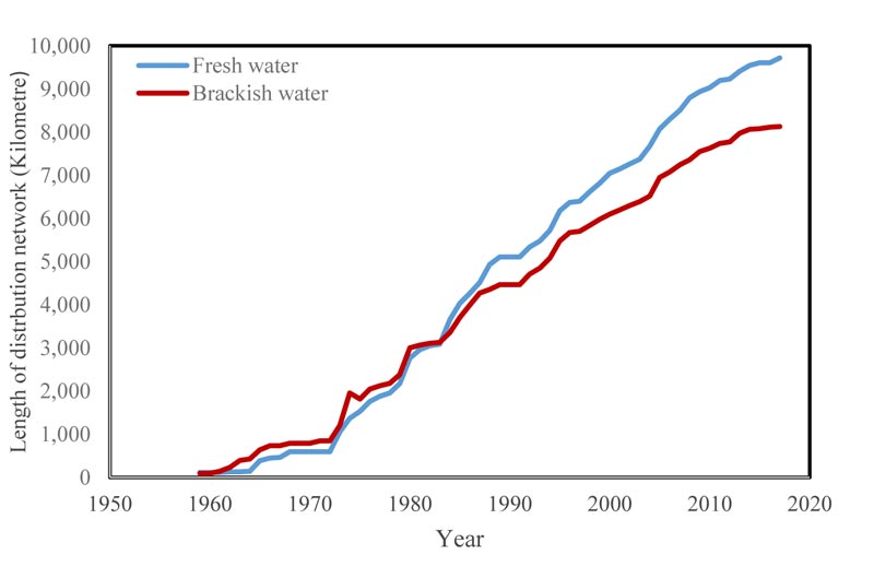
The water distribution network pipes are mainly ductile iron with few steel coated pipes. The diameter of the pipes is 3/4, 1 and 2 inches for household dwellings, commercial and industrial establishments, respectively. The total fresh water consumption has increased from 3 × 10⁶ m3 in the year 1957 to 160 × 109 m3 in the year 2018, which represents, in 60 years, a 53,000 folds increased. Tremendous changes had occurred to the fresh water distribution network over the years, from just 112 kilometers in length in 1959 to over 9,800 kilometers in 2018. Similarly, the brackish water distribution network had increased from 90 kilometers long in 1959 to over 8,100 kilometers in 2018. Moreover, the number of consumers connected to the fresh water network totaled 177,118 and consumers connected to the brackish water network totaled 77,257 by the end of 2018. However, there were 1,416 and 183 pipe breaks for the fresh water and brackish water, respectively. Fig. (1) shows the development of both the fresh and brackish water distribution networks in Kuwait from 1959 to 2018 [15-18].
3. RESULTS AND DISCUSSION
3.1. Formulation of the Models and Discussion of the Results
3.1.1. Case Study I (Pipe Breaks)
Hydraulic simulation of water distribution systems to forecast the future pressures and flow has been developed and implemented in the last two decades [19, 20]. However, the system simulation to predict the future pipe break pattern and future performance of the system to provide an uninterrupted water supply to its customers is in the developing stage at the present time [21, 22].
A water supply system typically consists of a source of water (e.g., reservoir, well, etc.), pumping stations, transmission conduit, storage reservoirs and a network of pipes making up the distribution system. Pipes break more frequently due to their underground concealment. Hence, they undergo more severe stresses, including, but not limited to, soil corrosiveness, frost penetration, overburden pressure and traffic loads. Furthermore, in most cases, pipes are not subject to preventive maintenance because their state of deterioration is invisible and unknown [23, 24].
Water main breaks are a problem of concern to many water supply agencies. Breaks cause disruption in service; pose a potential danger when they temporarily reduce firefighting capabilities; may cause damage to other services and to property; and, incur substantial repair cost.
At present, the problem of pipe breaks is mostly approached on a “react to crisis” basis in which pipes are repaired after they are broken. In this approach, only the broken pipes are repaired, and those which are about to break in the near future, are left untouched. In spite of this supposedly conventional wisdom, this may not be the best strategy. Such a strategy could be partly attributed to the lack of quantitative documentation to convince the decision-makers of the urgency of a preventive maintenance program [25, 26].
This case study shows how the data of pipe breakage is applied in order to forecast the future operations and preventive
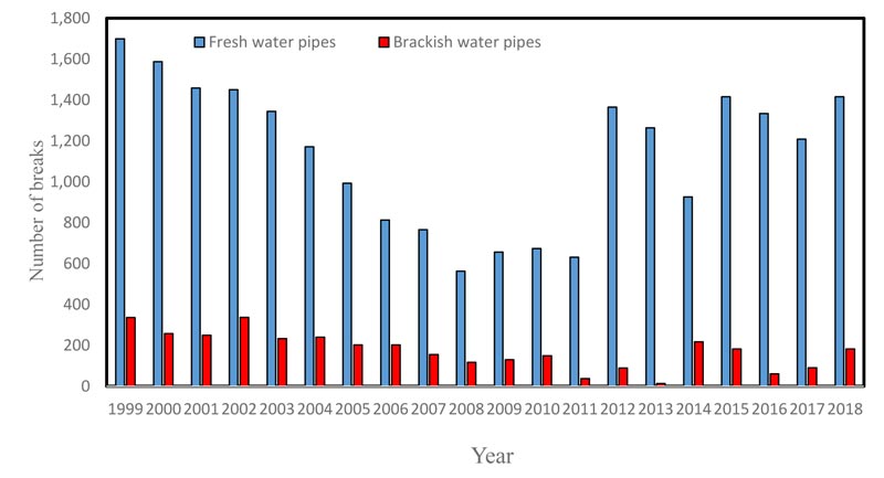
maintenance requirements of a water distribution system. The methodology is based on the Box-Jenkins approach of time series analysis [2]. Kuwait water system's database [15] was analyzed, from the database, the number of breaks occurring each year from 1999 to 2019 in pipes of different diameters and lengths was determined. The data are the monthly water main breaks; these water mains range in diameter from 50 mm (2 inches) to 300 mm (12 inches). Fig. (2) illustrates the yearly pipe break pattern from 1999 to 2018. It is noticed that the number of fresh water pipe breaks is by far higher than the brackish water pipe breaks, that is due to the higher use and consumption of fresh water in daily uses. In addition, brackish water is available for customers once a week only [15].
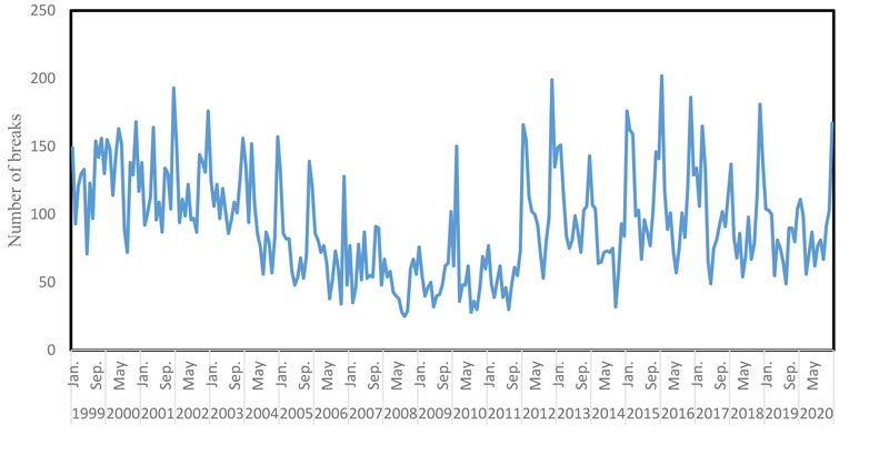
Fig. (3) shows the time series of the data. The symbols in the figure are used to specify the month for each observation. From Fig. (3), one can conclude that the number of water main breaks is highest during the winter months (December, January and February) due to the cold weather, and during the summer months (July and August) due to the increasing demand of water usage during these months. In Kuwait’s water break data, we find that the series completes an up-and-down cycle every 12 months. A series of this shape is said to be seasonal, where the period of seasonality in this case study happens to be 12 months.
| To Lag | Chi-Square | DF | Pr > Chi-Sq | Autocorrelation | |||||
|---|---|---|---|---|---|---|---|---|---|
| 6 | 353.1 | 6 | <0.0001 | 0.59 | 0.49 | 0.47 | 0.49 | 0.45 | 0.41 |
| 12 | 644.5 | 12 | <0.0001 | 0.44 | 0.45 | 0.47 | 0.42 | 0.42 | 0.42 |
| 18 | 798.2 | 18 | <0.0001 | 0.34 | 0.31 | 0.34 | 0.28 | 0.28 | 0.31 |
| 24 | 957.1 | 24 | <0.0001 | 0.36 | 0.38 | 0.25 | 0.24 | 0.30 | 0.33 |
| To Lag | Chi-Square | DF | Pr > Chi-Sq | Autocorrelation | |||||
|---|---|---|---|---|---|---|---|---|---|
| 6 | 2.27 | 2 | 0.3210 | 0.00 | 0.00 | 0.03 | 0.06 | 0.02 | 0.07 |
| 12 | 7.00 | 8 | 0.5369 | 0.00 | 0.01 | 0.11 | 0.01 | 0.02 | 0.07 |
| 18 | 16.63 | 14 | 0.2763 | 0.08 | 0.11 | 0.00 | 0.11 | 0.07 | 0.02 |
| 24 | 32.63 | 20 | 0.0570 | 0.05 | 0.14 | 0.11 | 0.10 | 0.04 | 0.11 |
| 30 | 38.44 | 26 | 0.0551 | 0.05 | 0.12 | 0.13 | 0.04 | 0.01 | 0.02 |
| 36 | 45.87 | 32 | 0.0533 | 0.05 | 0.04 | 0.04 | 0.01 | 0.10 | 0.05 |
| 42 | 50.67 | 38 | 0.0819 | 0.04 | 0.07 | 0.07 | 0.09 | 0.01 | 0.03 |
From the results of the analysis of the time series, we obtain the following model (Eq. 2) for the water main breaks data:
 |
(2) |
where;
Y(t) =The original water main break variable,
B = Backshift operator,
a(t)=The independent random error with constant variance.
It is clear from the time series analyses (Tables 1 and 2) that the data are highly correlated, since all the Pr values in Table 1 are less than 0.05. It is a good indication that means the present values in the time series are related to its past values. In addition, the Pr values of the residuals (Table 2) are all higher than 0.05. All this proves that the model is a good fit for the data.
3.1.2. Case Study II (Rainfall)
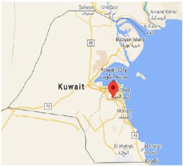
In this paper, the Box-Jenkins approach of time series analysis was applied on a set of daily rainfall data collected during a ten-year period from the seventh ring road disposal facility of the Municipality of Kuwait. The seventh ring road landfill is located about 30 kilometers (18.64 miles) southwest of Kuwait city, and comprised of 3 km2 (741.4 acres) (Fig. 4). Of this, 2.5 km2 is dedicated to landfilling, with the remaining area used as a buffer zone. The tonnage received at the facility is estimated as 210 tons/day of municipal solid wastes in 2018. Hydrologically, the effects of the Kuwait Bay on the climate pattern of the area are evidenced in the seasonal as well as temporal behavior of precipitation [15].
The importance of modeling (and forecasting) rainfall at solid wastes disposal sites stems from the urgent need for a reliable prediction of landfill leachate generation rates and quality [27-29]. The amount of leachate produced from a municipal landfill is a function of the quantity of water received by the landfill. Infiltrating precipitation into landfills is regarded as the major source of leachate [30, 31]. Table 3 shows the water quality results from water wells within the landfill site. However, a fraction of precipitation over a landfill site results in surface runoff, another fraction is lost back to the atmosphere in the form of evapotranspiration, and the remaining fraction adds to the moisture storage in the cover of the landfill or accesses into the refuse mass [32, 33].
| Parameter/Location | 1 | 2 | 3 | 4 |
|---|---|---|---|---|
| Depth of well (m) | 6 | 6.5 | 7 | 8 |
| Distance from landfill (m) | 2000 | 4395 | 4625 | 5000 |
| pH | 7.50 | 7.20 | 7.74 | 7.40 |
| Turbidity (JTU) | 3.80 | 10.20 | 296.6 | 4.80 |
| BOD (mg/l) | 11.20 | 17.20 | 338.0 | 6.00 |
| COD (mg/l) | 396.46 | 65.43 | 643.8 | 32.94 |
| Nitrate (mg/l) | 7.20 | 2.52 | 34.00 | 34.70 |
| Hardness (mg/l) | 5490.0 | 2800.0 | 10460.0 | 2386.0 |
| Total dissolved solids (mg/l) | 15.26 | 5.84 | 20.42 | 3.88 |

Conceptually, the leachate quantity generated at a sanitary landfill is proportionally correlated with the precipitation received at the site, and the proportionality coefficient is often incorporated as a site-specific coefficient. Accordingly, any successful attempt for modeling landfill leachate must be constructed on accurate estimations of the local rainfall data.
The fifty-eight year daily rainfall data, however, was averaged on a yearly basis, and the monthly averages of daily rainfall for the period of 1962 to 2019 were obtained. The new set of data
Fig. (5) was then analyzed via the P2T programming of the BMDP and SAS statistical software packages [13, 14]. Fig. (4) represents the time series of the yearly averages of daily rainfall measurements at the seven ring road solid waste management facilities. This time series indicates considerable variations in the precipitation values from less than 0.001 mm/d to about 0.312 mm/d, nevertheless, it shows the seasonal, cyclical distribution of the observed data.
The analysis, carried out with the aid of the BMDP package, revealed the pertinent features of the rainfall measurements, and provided an explicit parametric model to facilitate the forecasting of future monthly values of rainfall as follows (Eq. 3):
 |
(3) |
where;
Y(t) = the original rainfall variable,
B = Back casting operator, and
a(t) = The random error variable.
| To Lag | Chi-Square | DF | Pr > Chi-Sq | Autocorrelation | |||||
|---|---|---|---|---|---|---|---|---|---|
| 6 | 17.44 | 6 | <0.0001 | 0.51 | 0.09 | 0.11 | 0.06 | 0.45 | 0.05 |
| 12 | 19.94 | 12 | <0.0001 | 0.04 | 0.10 | 0.13 | 0.01 | 0.42 | 0.06 |
| 18 | 25.56 | 18 | <0.0268 | 0.03 | 0.00 | 0.05 | 0.02 | 0.28 | 0.19 |
| 24 | 39.08 | 24 | <0.0683 | 0.15 | 0.14 | 0.17 | 0.08 | 0.31 | 0.22 |
| To Lag | Chi-Square | DF | Pr > Chi-Sq | Autocorrelation | |||||
|---|---|---|---|---|---|---|---|---|---|
| 6 | 0.72 | 6 | <0.0068 | 0.01 | 0.03 | 0.03 | 0.06 | 0.03 | 0.05 |
| 12 | 4.57 | 12 | <0.0080 | 0.02 | 0.04 | 0.09 | 0.01 | 0.11 | 0.16 |
| 18 | 8.30 | 18 | <0.0087 | 0.06 | 0.08 | 0.12 | 0.01 | 0.08 | 0.11 |
| 24 | 12.88 | 24 | <0.0088 | 0.05 | 0.00 | 0.18 | 0.05 | 0.04 | 0.07 |
It is apparent from the forecasting model that the yearly frequency of the rainfall data is the main contributor to the non-stationary and variable behavior of the time series. The forecasted values of the monthly average of daily rainfall are illustrated in Fig. (4), which confirms higher precipitation rates during the spring and fall seasons. Moreover, it is clear from the time series analyses (Tables 4 and 5) that the data are highly correlated, since all the Pr values in Table 1 are less than 0.05. That is a good indication, which means that the present values in the time series are related to its past values. In addition, the Pr values of the residuals (Table 5) are all higher than 0.05. All this proves that the model is a good fit for the data.
Consequently, the forecasting procedure, as presented, can be incorporated with other hydrologic models in order to predict the net percolation rates of precipitation into the landfill and virtually used to predict and estimate the leachate generation rate at this specific landfill. Although the overall modeling procedure of landfill leachate is beyond the aim of this paper, it is of importance to mention that the Box-Jenkins analysis of time series was incorporated in the hydrologic simulation of landfills and namely in the PITTLEACH model of sanitary landfills leaching and stabilization [33-35]. The PITILEACH model utilizes the forecast rainfall data and estimates the external moisture flux into the landfill by multiplying these values by a proportionality factor (of a magnitude = 0.05-0.12). Thereafter, principles of flow dynamics in porous media, as well as the theory of unsaturated transport, facilitate the prediction of landfill leachate rates. Furthermore, the simulation results of these models are the basis upon which design, operational and closure plans are decided.
CONCLUSION
Two explicit parametric models were developed herein to forecast the future (and present) trends and values of two sets of observation data. These observations represent the hydraulic failure of an engineered system (pipe break in water networks), and the behavior of a natural system (precipitation on solid waste disposal sites). The analyses were conducted by the applications of the time domain approach of time series analysis. The usefulness of this probabilistic was evidenced not only in its simplicity and modeling capability, but also in its demonstrated flexibility to complement various simulation efforts. In the first and second study cases of pipe breaks and rainfall, respectively, the data were highly correlated. All the Pr values were less than 0.05, which means that the present values in the time series are related to its past values. In addition, the Pr values of the residuals were all higher than 0.05. All this proves that the model is a good fit for the data. The results showed a significant correlation between the data and the time series models provides good estimates of pipe reliability and rainfall measurements. Therefore, it could be useful for water authorities in planning pipe maintenance and inspection.
It is recommended and it would be very useful to conduct similar studies on pipes carrying other fluids such as gas, air and oil.
CONSENT FOR PUBLICATION
Not applicable.
AVAILABILITY OF DATA AND MATERIALS
The data sets analyzed during the current study are available from the corresponding author [J. A] upon request.
FUNDING
None.
CONFLICT OF INTEREST
The authors declare no conflict of interest, financial or otherwise.
ACKNOWLEDGEMENTS
The authors are very thankful to the distinguished reviewers of the journal for their insightful comments and suggestions.

