All published articles of this journal are available on ScienceDirect.

Application of a Genetic Algorithm for the Optimal Calibration of Hysteretic Models
Abstract
Background:
Recent computing improvements have allowed a considerable use of numerical models to predict phenomena concerning various topics. In particular, considering the field of civil engineering, the possibility of having greater computational capabilities has guaranteed to explore both the global and local behaviour of buildings with greater attention and precision so that currently, many software programs allow modelling different structural components with high accuracy.
Objective:
One of the aspects of interest concerns the calibration of phenomenological laws to model the mechanical behaviour of specific structural members, devices or connections. With this in mind, many efforts have recently been dedicated to solving this problem by implementing computational codes called “Genetic Algorithms”, which provide optimal configurations of parameters following procedures that emulate Darwin’s theory of evolution. However, generally, these algorithms are encoded in C++ formats, which are difficult to be modified basing on the needs of the users.
With this in mind, the present work's novelty consists of implementing a Genetic Algorithm that, starting from the knowledge of assigned hysteretic curves, allows their modelling through an appropriate calibration of the parameters of the “hysteretic” uniaxialmaterial element of the OpenSees software. In particular, the originality of the code proposed in this paper is its development in the Matlab environment, which is more easily editable and more flexible to customers' specific needs than traditional C++ compilers, such as MultiCal, a calibration software already available in research.
Methods:
Genetic Algorithms are instructions through which it is possible to reach the optimal calibration of mathematical models according to a procedure that conceptually refers to the evolutionary process of living species.
Results:
The proposed GA has been validated against MultiCal tool by calibrating 44 force-displacement hysteretic curves obtained from finite element simulations relating to the cyclic behaviour of connections between circular hollow section profiles and passing-through plates subjected to displacement histories in the axial direction.
Conclusion:
The results have shown that the proposed algorithm calibrates the known responses with acceptable accuracy, in line with or even better than the outcomes provided by MultiCal.
1. INTRODUCTION
The technological developments that occurred in the last decades have profoundly impacted our society, promoting enhancements in several areas, including civil engineering. In particular, the increased computational capacities in this field widened the topics to be investigated, with specific attention to advanced Finite Element (FE) analyses accounting for complex non-linearities at the materials, sections, members and devices level. This modelling approach relies on the basis that the current seismic provisions require designing structures able to dissipate the seismic input energy in well-defined and known a priori elements. Consequently, the non-linearities can be modelled through zero- or finite-length elements, assigning an elastic behaviour to the other structural parts [1, 2].
Under this perspective, the enhancements of the computational capacities have allowed exploiting a comprehensive collection of non-linear models which differ in the degree of sophistication; for clarity, it is worth mentioning the most relevant mathematical implementations currently embedded in structural software: Ramberg and Osgood [3], Bouc and Wen [4, 5], Takeda [6], Richard and Abbott [7], Dowell, Seible and Wilson [8], Sivaselvan and Reinhorn [9], Ibarra, Medina and Krawinkler [10]. However, also other more simple models are available, like the traditional bilinear elastic-plastic law (implemented, for instance, as “Steel01” in OpenSees [11] or “bl_sym” in SeismoStruct [12]).
The parameters of the non-linear models mentioned above have mainly a phenomenological significance rather than a mechanical meaning. Nevertheless, their primary merit is the possibility of characterising experimental stress-strain, force-displacement or moment-rotation responses, even ignoring the physical connotations on which the observed phenomena rely. Therefore, the calibration of these phenomenological models against known responses represents a fundamental step towards their effective exploitation in common structural software. In particular, this purpose can be achieved by following three strategies:
(1) Choosing only the simple models whose parameters can be defined by relying on physical evidence (the limit of this alternative is the restriction of the proposed models' application fields);
(2) Calibrating the sophisticated models randomly varying their parameters until an acceptable configuration is achieved (this strategy is computationally expensive without relying on any optimisation basis);
(3) Implementing a programmed calculation routine based on Genetic Algorithms (GAs) that identifies and optimises the parameters that better replicate the known non-linear response.
The last approach represents the best alternative because it has the merit of calibrating the parameters of every phenomenological model speeding up the process and significantly limiting the randomness search. Genetic Algorithms (GAs) represent a transposition of Darwin's theory of species evolution to the computing field, intending to optimise the calibration of mathematical laws belonging to the most diversified subjects. The first application of this technique concerned the biology field and happened in 1975 by Holland [13]. Instead, the introduction to civil engineering occurred in 1986 by Goldberg and Samtani [14]. Pezeshk et al. [15] proposed the first genetic routine for the optimal design of 2D steel structures, while Del Savio et al. [16] and Cheng [17] promoted genetic codes to design steel structures with semi-rigid joints and arch bridges with tie rods and steel towers, respectively. Furthermore, Falcone et al. proposed a rational selection procedure based on GAs for the seismic retrofitting of existing reinforced concrete structures [18] by introducing concentric X-shaped steel bracings or FRP jacketing of columns.
The strategy based on GAs has also been applied for the automatic calibration of hysteretic structural models through the development of the MultiCal (Multi-objective Calibration) tool [19]. It has been conceived to achieve a multi-objective optimisation of many phenomenological models implemented in OpenSees [11] and SeismoStruct [12], minimising the following quantities: generalized stress (or force or moment) history, energy history, and envelope curve. MultiCal tool has been widely tested [19], showing its reliability for the calibration of monotonic or cyclic curves and in the case of hysteretic responses characterized by non-standardised loading patterns (this is the case of outcomes by pseudo-dynamic tests [19]). Nevertheless, since MultiCal is developed in C++ [20], special technical knowledge is required to read or modify the source code. Furthermore, the optimisation process employs a one-single core of the CPU, slowing down the procedure.
This paper proposes an integrated numerical procedure between Matlab and OpenSees for calibrating the parameters of the “hysteretic uniaxialmaterial” element belonging to the OpenSees library through a simple Genetic Algorithm. In particular, the effectiveness of the proposed solution is demonstrated by applying the developed routine to 44 cyclic force-displacement curves, which represent the results of Abaqus simulations concerning connections between Circular-Hollow-Section (CHS) profiles and through-all axially loaded plates. Nevertheless, unlike MultiCal, the proposed algorithm has been implemented to optimise only the generalized force-displacement responses, neglecting the optimisation in terms of energy and envelope. Consequently, the objective is achieved by minimising the sum of the squared normalized scatters among the known and predicted forces along the hysteretic curves.
Finally, the same 44 curves have been calibrated employing the MultiCal tool and compared with the proposed GA's corresponding outcomes, demonstrating the implemented routine's satisfactory accuracy.
2. METHODOLOGY
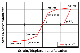
The present work aims to propose a simple Genetic Algorithm to define the parameters (Table 1) of the OpenSees “hysteretic uniaxialmaterial” model (Fig. 1) for the calibration of cyclic stress-strain, force-displacement or moment-rotation curves.
| Parameters | - |
|---|---|
| s1p and e1p | Force and displacement at 1st point of the envelope in the positive direction |
| s2p and e2p | Force and displacement at 2nd point of the envelope in the positive direction |
| s3p and e3p | Force and displacement at 3rd point of the envelope in the positive direction |
| s1n and e1n | Force and displacement at 1st point of the envelope in the negative direction |
| s2n and e2n | Force and displacement at 2nd point of the envelope in the negative direction |
| s3n and e3n | Force and displacement at 3rd point of the envelope in the negative direction |
| pinchx | Pinching factor for deformation during reloading |
| pinchy | Pinching factor for force during reloading |
| damage1 | Damage due to ductility |
| damage2 | Damage due to energy |
| beta | Power used to determine the degraded unloading stiffness based on ductility |
In particular, the paper intends to test the GA against 44 cyclic force-displacement hysteretic curves obtained by Finite Element (FE) simulations performed on connections between circular-hollow-section profiles and through-all axially loaded plates (Fig. 2). Before performing these analyses, the FE model, developed in Abaqus, was validated against three monotonic and three cyclic experimental tests [21, 22].
These results belong to a more extensive research program currently ongoing at the University of Salerno concerning the component characterization of joints between CHS columns and through-all double-tee profiles.
Table 2 shows the methodology applied to implement and validate the proposed Genetic Algorithm, summarising the research's main steps and associating them with the paragraphs of the present paper.
| Step AInvestigated Cases | Step BProposed Genetic Algorithm (GA) | Step CReliability of the Proposed GA |
|---|---|---|
| -Experimental activity-Finite Element Modelling-Parametric analysis | -Implementation of the GA | -Application of the GA to calibrate 44 cyclic force-displacement curves-Assessment of the reliability of the proposed GA through the comparison with the MultiCal tool |
Step A (paragraph 3) discusses the experimental activity, the Finite Element (FE) modelling and the parametric analysis performed on connections between CHS columns and passing-through plates. This section's main aim is to create a large database composed of 44 force-displacement hysteretic curves that can be exploited to assess the effectiveness of the proposed code.
Step B (paragraph 4) reports a detailed description of the implemented algorithm discussing the main parameters affecting its response, the variable intended to be optimised and retraces all the main stages of the procedure through a logical flow.
Step C (paragraph 5) deals with the application of the GA to the cases selected in paragraph 3 and assesses its reliability by comparing the outcomes of its calibrations against analogous results obtained by adopting the MultiCal tool.
3. CASE STUDY
This paragraph provides information about the experimental and numerical activities on connections between tubular profiles and through-all plates in order to create a database of 44 force-displacement curves that are essential to test the reliability of the proposed GA.
3.1. Experimental Activity
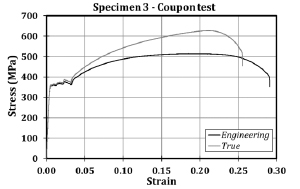
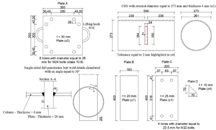
As anticipated, three cyclic tests on Circular-Hollow-Section (CHS) to through-all plate connections have been performed at the STRENGTH Laboratory of the University of Salerno. The geometrical properties of the tested specimens are reported in Table 3. This selection is motivated by the need to test Circular Hollow Section to through-all plate connections representative of the flanges of double-tee profiles belonging to tubular to passing-through I-beam joints. In particular, the chosen plates correspond to the flanges of the IPE200, IPE300 and IPE330 sections. Furthermore, as demonstrated by coupon tests (Fig. 3), all the elements were made of S355JR steel grade.
The hollow profiles have been cut with a tolerance of 2 mm so that single-sided full-penetration welds chamfered with an angle equal to 30° could be manufactured (Fig. 4).
| - | Circular Hollow Section | Through-all Plate | ||||
|---|---|---|---|---|---|---|
| Specimen | External diameter (mm) | Thickness (mm) | Length (mm) | Width (mm) | Thickness (mm) | Length (mm) |
| 1 | 168.0 | 6.0 | 450.0 | 100.0 | 30.0 | 350.0 |
| 2 | 219.1 | 5.0 | 500.0 | 150.0 | 20.0 | 350.0 |
| 3 | 273.0 | 6.0 | 500.0 | 160.0 | 20.0 | 400.0 |
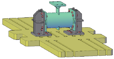
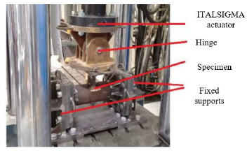
The tests have been performed by applying cyclic displacements at the upper end of the plates using a vertical actuator characterised by a loading capacity of 2000 kN in tension and 3000 kN in compression. In addition, fixed constraints have been applied to the ends of the tubular profiles employing rigid supports (Fig. 5). The cyclic tests have been performed by adapting the AISC 341-16 loading protocol [23] for beam-to-column connections to the examined cases, as reported in Table 4. Furthermore, the displacements have been applied, setting the rate to values equal to 0.5 mm/min, 1 mm/min, and 2 mm/min for the ranges 0-10 mm, 10-20 mm and higher than 20 mm, respectively.
| - | Amplitudes (mm) | ||
|---|---|---|---|
| n. cycles | Test 1 | Test 2 | Test 3 |
| 6 | 0.75 | 1.125 | 1.2 |
| 6 | 1 | 1.5 | 1.6 |
| 6 | 1.5 | 2.25 | 2.4 |
| 4 | 2 | 3 | 3.2 |
| 2 | 3 | 4.5 | 4.8 |
| 2 | 4 | 6 | 6.4 |
| 2 | 6 | 9 | 9.6 |
| 2 | 8 | 12 | 12.8 |
| 2 | 10 | 15 | 16 |
| 2 | 12 | - | - |
| 2 | 14 | - | - |
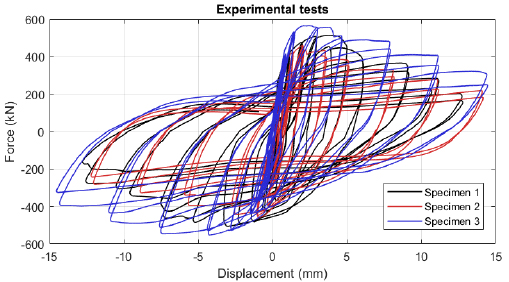
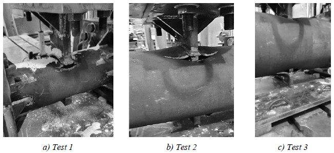
The force-displacement curves of the tested specimens are shown in Fig. (6). The maximum strength withstood by the three specimens was equal to 515 kN, 462 kN and 565 kN, respectively, and has been achieved for displacements lower than 5 mm in all cases, highlighting the low deformation capacity of the analysed component. Moreover, after achieving the peak resistance, the three responses are characterised by a softening behaviour induced by the residual resistance offered by the local crushing and tearing observed, respectively, at the upper and lower tube-to-plate attachments. The consequences of this statement are demonstrated by the damages experienced by the specimens and shown in Fig. (7).
3.2. Finite Element (FE) Modelling
Finite Element (FE) models of the tested specimens have been developed with the software Abaqus. The geometrical properties have been accurately modelled with the only exception of the welds, which have been simplified by adopting “tie” contacts between the connected elements. Referring to the results of coupon tests, the constitutive material law has been defined by employing a quadrilinear stress-strain curve, as suggested by Faella et al. [24].
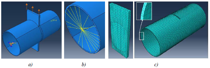
Since the fixed supports of the experimental set-up are rigid, only the CHS to through-plate specimens have been modelled (Fig. 8). “Coupling” constraints (Fig. 8) connect the tubular ends to their sections’ centres, which have been fixed through external restraints, while the same displacement histories experienced by the three specimens at the end of the plates have also been applied to the numerical models.
The developed models account for the spread of damage through an evolution law, whose parameters have been defined on the results provided by Faralli et al. [25] and Pavlovic et al. [26], using a mesh size of 5 mm (Fig. 8) with 8-node linear brick type (or C3D8 type) elements for all the members.
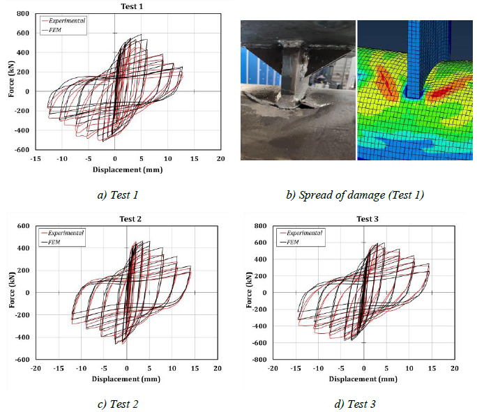
The numerical models have been validated against the experimental results, as shown in Fig. (9), where the comparisons of the force-displacement curves and failure modes exhibited by the tested specimens and FE simulations are reported. Furthermore, the maximum strength exhibited by the analysed specimens during the experimental activities and the numerical simulations are reported and compared in Table 5; it is possible to establish that the proposed numerical models have been validated against the experimental results since the maximum observed scatter is below 14%.
| Maximum Strength (kN) | Specimen 1 | Specimen 2 | Specimen 3 |
|---|---|---|---|
| Experimental | 515 | 462 | 565 |
| FEM | 587 | 466 | 597 |
| Scatter (%) | +14 | +1 | +6 |
| Test | d0 (mm) | t0 (mm) | b1 (mm) | tp (mm) | Test | d0 (mm) | t0 (mm) | b1 (mm) | tp (mm) |
|---|---|---|---|---|---|---|---|---|---|
| 1 | 193.7 | 6 | 120 | 20 | 23 | 193.7 | 6 | 125 | 25 |
| 2 | 193.7 | 6 | 120 | 22.5 | 24 | 193.7 | 6 | 130 | 25 |
| 3 | 193.7 | 6 | 120 | 25 | 25 | 219.1 | 4 | 120 | 25 |
| 4 | 193.7 | 6 | 120 | 30 | 26 | 219.1 | 4 | 130 | 25 |
| 5 | 193.7 | 6 | 120 | 35 | 27 | 219.1 | 4 | 140 | 25 |
| 6 | 219.1 | 4 | 150 | 15 | 28 | 219.1 | 4 | 150 | 25 |
| 7 | 219.1 | 4 | 150 | 20 | 29 | 219.1 | 4 | 160 | 25 |
| 8 | 219.1 | 4 | 150 | 25 | 30 | 244.5 | 8 | 140 | 25 |
| 9 | 219.1 | 4 | 150 | 30 | 31 | 244.5 | 8 | 150 | 25 |
| 10 | 219.1 | 4 | 150 | 35 | 32 | 244.5 | 8 | 160 | 25 |
| 11 | 244.5 | 8 | 160 | 25 | 33 | 244.5 | 8 | 170 | 25 |
| 12 | 244.5 | 8 | 160 | 30 | 34 | 244.5 | 8 | 180 | 25 |
| 13 | 244.5 | 8 | 160 | 32.5 | 35 | 406.4 | 10 | 180 | 25 |
| 14 | 244.5 | 8 | 160 | 35 | 36 | 406.4 | 10 | 190 | 25 |
| 15 | 244.5 | 8 | 160 | 40 | 37 | 406.4 | 10 | 200 | 25 |
| 16 | 406.4 | 10 | 200 | 20 | 38 | 406.4 | 10 | 210 | 25 |
| 17 | 406.4 | 10 | 200 | 25 | 39 | 406.4 | 10 | 220 | 25 |
| 18 | 406.4 | 10 | 200 | 35 | 40 | 219.1 | 4 | 120 | 20 |
| 19 | 193.7 | 6 | 105 | 25 | 41 | 219.1 | 4.5 | 120 | 22.5 |
| 20 | 193.7 | 6 | 110 | 25 | 42 | 219.1 | 5 | 120 | 25 |
| 21 | 193.7 | 6 | 115 | 25 | 43 | 219.1 | 5.5 | 120 | 27.5 |
| 22 | 193.7 | 6 | 120 | 25 | 44 | 219.1 | 6.5 | 120 | 32.5 |
3.3. Parametric Analysis
The validation of the FE model developed in Abaqus has been exploited to perform a parametric analysis to extend the studied configurations of CHS to passing-through plate connections. In particular, 44 different geometric combinations of S355JR steel grade tubular profiles and plates have been selected (Table 6) by varying the diameter of the tube between 193.7 mm and 406.4 mm, the thickness of the tube between 4 mm ad 10 mm, the plate width between 105 mm and 220 mm and, finally, the thickness of the plate between 15 mm and 40 mm.
The simulations have been carried out by adopting a static solver and applying cyclic displacement histories at the ends of the plates complying with the AISC 341-16 loading protocol [23].
4. IMPLEMENTATION OF THE GENETIC ALGORITHM
4.1. General Description
Genetic Algorithms (GAs) represent an interesting solution to be adopted in the case of optimisation problems since they are conceived to calibrate the modelling parameters of mathematical laws to achieve the best fitting of experimental data. The implementation of the GAs evokes Darwin’s theory of evolution. In fact, living beings result from an evolutionary process mainly governed by random variabilities that have allowed the survival only of those individuals characterized by the strongest capacities.
Genetic Algorithms intend to transpose this approach in the computational field, optimising multiple parameters that can affect a model. The search for the optimal configuration of parameters starts with the preliminary random generation of individuals whose “survival skills” (which correspond to the fitting with the experimental response) are assessed through an appropriate Fitness-Function. This function is the selective operator for identifying the best individuals concerning the analysed generation. In the subsequent step, these individuals are employed to create new individuals for the successive generation. This approach is replicated over the generations, embedding random mutation and cross-over operators in the evolutionary process. The main steps of a GA are the following.
1) Definition of the input parameters
The number of individuals created during each generation, the number of generations and the first individual, are the input parameters of a GA. It is worth highlighting that the first individual can be selected by assigning random values to the configuration parameters, provided that they allow the mathematical law to be run.
2) Generations: procedure and operators
Starting from the best individuals of the previous generation, the random mutation and cross-over operators are used to generate the new individuals. The mutation randomly modifies the values assumed by the parameters of the last best individual. The cross-over creates new individuals by switching the values of parameters belonging to different previous optimal solutions.
3) Running of the mathematical law with the selected individuals
Testing of the configurations of parameters selected in the previous step.
4) Post-processing of the results and application of the Fitness-Function
The results are extracted, and a function (Fitness-Function) to evaluate how the model with the proposed parameters fits the experimental response is defined.
5) Selection of the best individual
The best individual is assessed and used for the subsequent generation.
4.2. Proposed Implementation
Considering the main characteristics reported above, the work of this paper has been focused on implementing in Matlab a genetic algorithm for the optimal calibration of the parameters concerning the “hysteretic uniaxialmaterial” model belonging to the OpenSees library [11].
This paragraph is entirely focused on the description of the proposed Genetic Algorithm, which, for clarity, will be denoted as pGA. The procedure adopted to perform the first generation of the pGA is reported in Fig. (10).
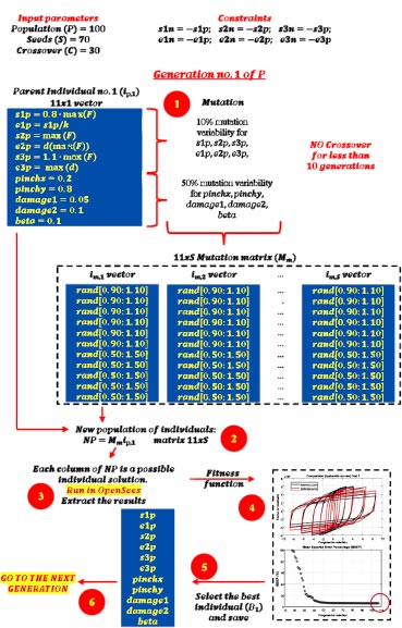
The input parameters are the population (P), the seeds (S) and the cross-over (C). P represents the number of generations to be created, S is the number of individuals produced through the mutation operator within each generation, and C represents the number of individuals created by applying the crossover operator. These parameters have been set equal to 100, 70 and 30, respectively. Moreover, observing the “Constraints” section reported in Fig. (10), the “hysteretic uniaxialmaterial” model has been forced to be symmetric.
To provide the initial values to s1p, e1p, s2p, e2p, s3p, e3p, it has been assumed that the envelope's first point coincides with the reference point curve where for the first time the 80% of the maximum resistance is attained. Instead, the second point of the envelope corresponds to the peak resistance. Finally, the third point of the envelope has been assumed as the point where the reference curve attains the maximum displacement. These formulations (shown in vector ip,1 of (Fig. 10) do not provide the correct values of the parameters, but they initialize the vector of the first individual. Instead, the parameters related to the pinchx, pinchy, damage1, damage2, beta have been set without searching for a physical meaning, respectively equal to 0.2, 0.8, 0.05, 0.1 and 0.1.
Step 1 of the pGA involves the generation of the first population of individuals. This scope can be achieved through the random mutation operator. As shown in Fig. (10), it has been assumed a mutation coefficient of 10% for parameters s1p, e1p, s2p, e2p, s3p, e3p, and a 50% coefficient for pinchx, pinchy, damage1, damage2, beta. This assumption means that the code generates a mutation matrix, Mm, with size 11 xS. The elements belonging to the first six rows randomly vary between 0.90 and 1.10, while the variation for the remaining rows is between 0.50 and 1.50. Considering that at this step, the cross-over operator cannot be applied since not enough solutions are available, the new population of individuals is assessed as NP = Mmip,1 (Step 2).
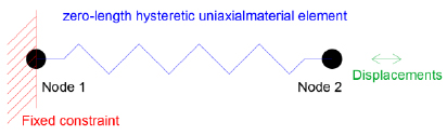
Each column of matrix NP represents a configuration of parameters of the “hysteretic uniaxialmaterial” element to be tested. In the third step, many OpenSees models run, having as input of the zero-length “hysteretic uniaxialmaterial” element in each column of NP and saving the numerical results for each analysed configuration. The OpenSees models have been conceived according to the scheme shown in Fig. (11): two coincident nodes are connected through a zero-length element characterised by the “hysteretic uniaxialmaterial” properties along the only x-direction. All the degrees of freedom of one node are fixed, while the displacement history is applied to the other node.
It is worth highlighting that the Matlab code has been implemented to be compatible with parallel computing so that several OpenSees models can run simultaneously on different cores (in this case, set equal to six) of the Central Processing Unit (CPU). This choice has been inspired by the need to speed up the optimisation procedure.
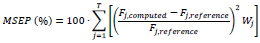
Then, by comparing the reference curve with the obtained numerical one, it is possible to define a Fitness Function that, in this case, corresponds to the Mean Squared Error Percentage (MSEP) over the steps of the input loading (Step 4). The mathematical formulation of the Fitness Function is reported in Eq. (1).
 |
(1) |
For clarity, T represents the number of discretised displacements’ values applied to the specimens, while Fj,computed and Fj,reference are the force values obtained by the OpenSees mathematical model and the numerically simulated specimen at the same j-th instant. Instead, Wj is a weighting factor which is equal to 0 if the absolute value of Fj,reference is lower than 10% of the maximum experimentally recorded force (Fj,reference,max), otherwise it linearly varies between 5 and 1 for j ranging between 1 and T. The introduction of factor Wj is justified by the need to neglect the excessive and meaningless errors which occur for low values of the denominator shown in Eq. (1) (Fj,reference). Furthermore, since many cycles with low amplitudes characterise the input histories, factor Wj allows amplifying the errors in the initial cycles of the hysteretic curve, otherwise, the influence of the last cycles prevails.
Finally, the best individual of the current generation is assessed in Step 5, and if its MSEP is lower than the initial solution, it becomes the new best individual (B1of Step 6), and it is used for the forthcoming generation.
The procedure adopted for the subsequent generations is similar to the scheme discussed above. For clarity, a schematic representation is reported in Fig. (12) for the generic i-th generation.
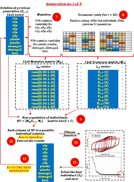
In this case, Step 6 is analogous to Step 1, with the only difference being that the generating vector corresponds to the individual selected in the previous step (Bi-1). Additionally, the cross-over operator is also applied (Step 8). It consists of a random switching among the values assumed by the parameters of the previous best ten solutions. This random mixture generates additional C individuals, collected into Mc matrix. In Step 9, the NP matrix is generated by collecting the MmBi-1 and Mc matrices. Then, Steps 10 to 13 are analogous to Steps 3 to 6. Obviously, if the optimal individual obtained in the i-th generation is better than Bi-1, then it is renamed as Bi, otherwise, Bi = Bi-1.
5. VALIDATION OF THE PROPOSED GENETIC ALGORITHM
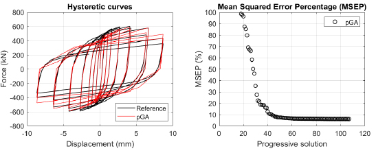
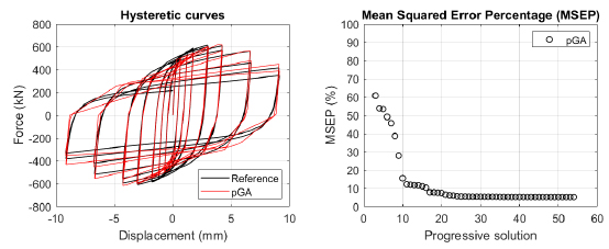
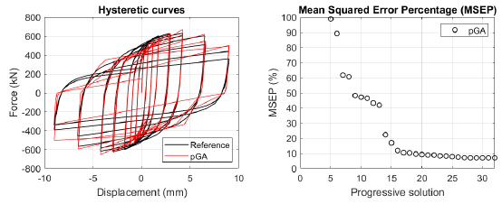
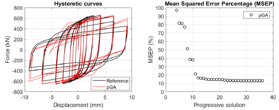
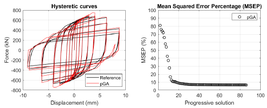
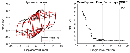
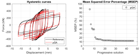
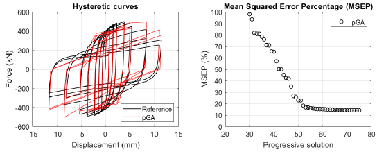
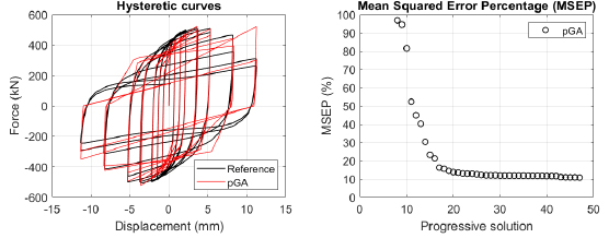
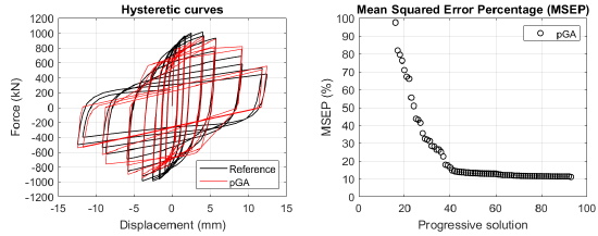
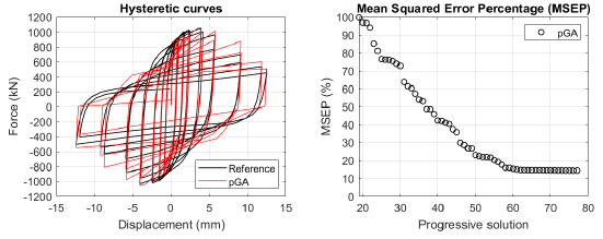
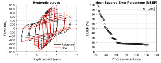
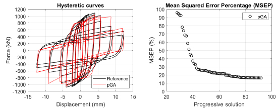
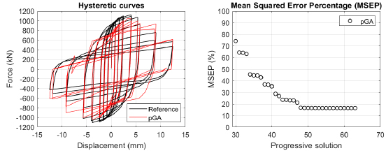
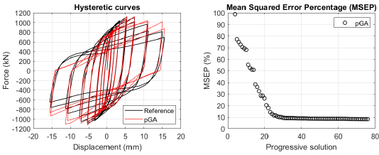
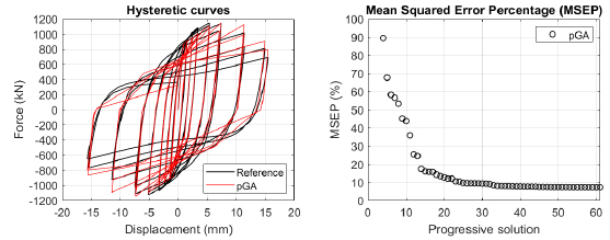
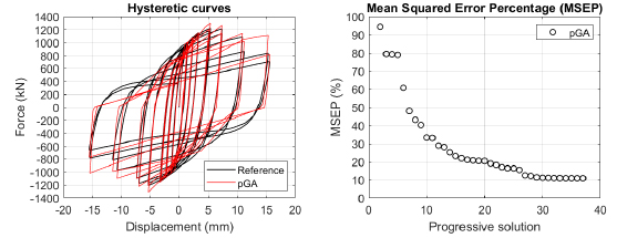
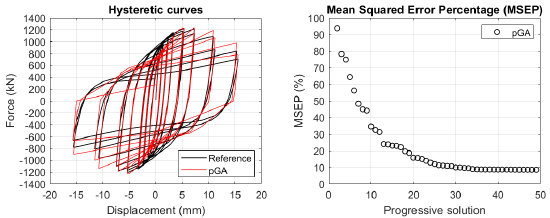
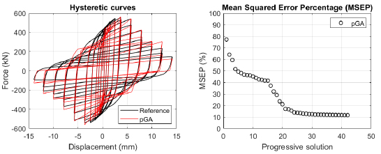
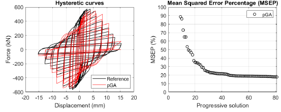
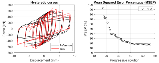
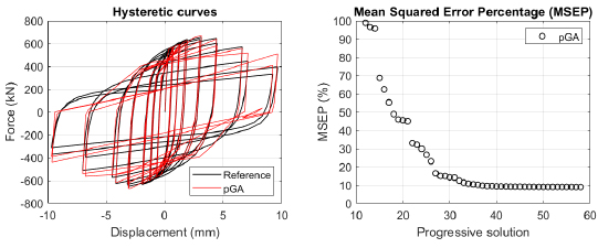
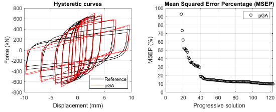
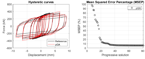
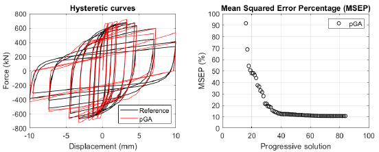
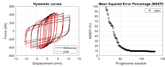
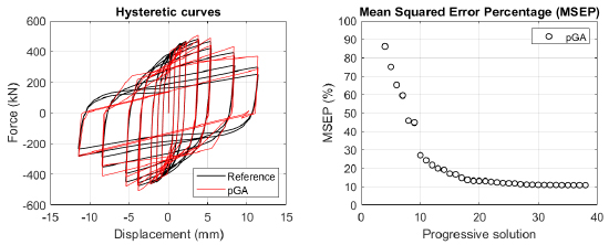
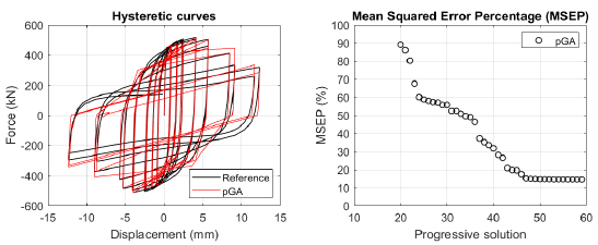
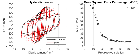
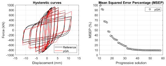
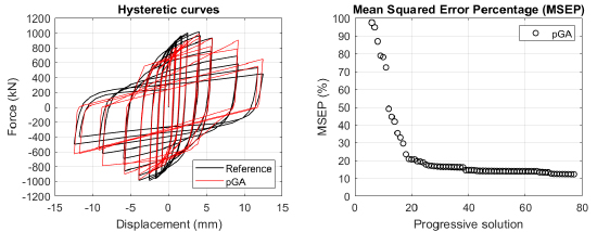
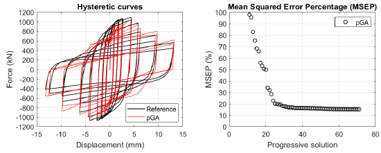
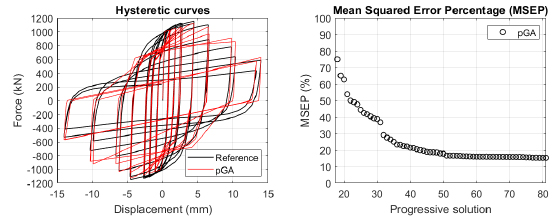
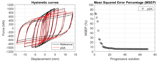
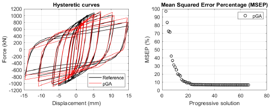
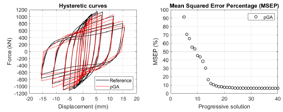
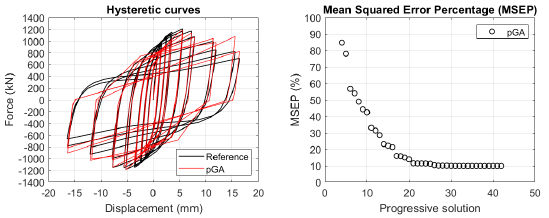
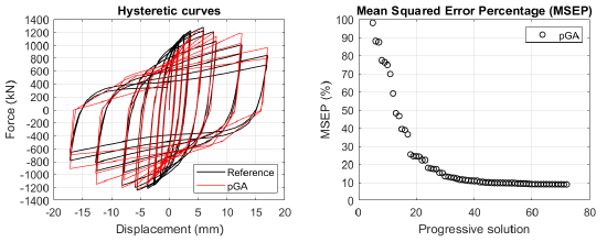
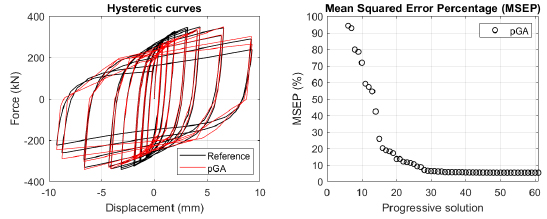
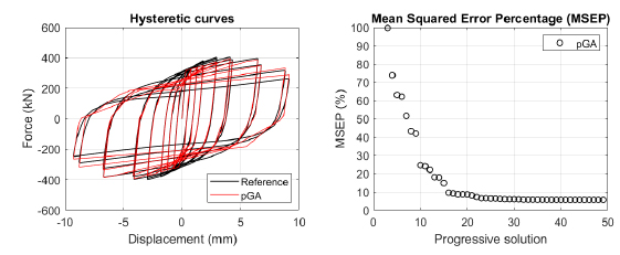
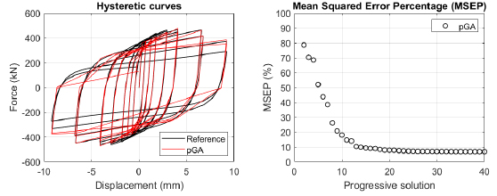
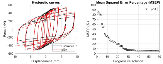
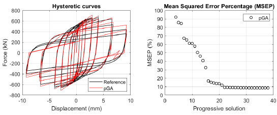
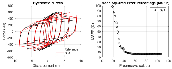
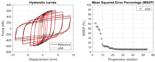
The algorithm described in paragraph 4 has been applied for calibrating the cyclic force-displacement curves of the 44 cases selected in paragraph 3. However, the results related to the first two cases are reported in Figs. (13, 14 and 16). The main outcomes are collected in the Annex (Figs. 17-60) of the paper.
| Proposed Genetic Algorithm (pGA) | MultiCal |
|---|---|
| More user-friendly implementation code since it is developed in Matlab | Code developed in C++ environment requires specialist knowledge to be understood |
| Process optimisation through multi-core analysis (faster process) | Single-core analysis (slower process) |
| No Multi-Objective calibration: only force optimization is implemented | Multi-Objective calibration: force, energy, envelope |
| Optimisation process applied only to the “hysteretic uniaxialmaterial” model (Opensees [11]) | Optimisation process applied to many models currently available in Opensees [11] and SeismoStruct [12] libraries |
| Better solutions than MultiCal in many cases of the analysed configurations of connections | - |
Generally, the proposed algorithm is able to predict with high precision the stiffness and maximum strength of the hysteretic responses. Moreover, the damage and softening envelope of the cycles are also foreseen with acceptable accuracy. For all the considered cases, the comparison between the force-displacement curves is always associated with the corresponding graph representing the Mean Squared Error Percentage and the progressive solutions that the algorithm defines over the generations. The analysed configurations highlight that a few dozen cases are needed to reach an acceptable solution; in fact, the MSEP graphs are characterized by a rapid reduction of the error at the very beginning of the running procedure. Nevertheless, the optimisation process goes on to find a better solution.
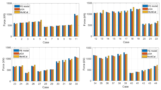
In order to validate the pGA, the same cases have been calibrated by employing the MultiCal tool applying the same inputs and disabling the energy and envelope objectives. The comparison in terms of maximum strength exhibited by the 44 analysed FE simulations and the corresponding calibrations are shown in Fig. (15).
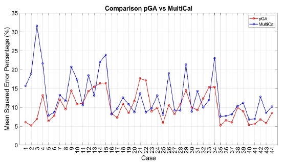
Finally, the Fitness Function defined in Eq. (1) has been applied to the optimised configurations of parameters selected for the 44 cases with the pGA and the MultiCal tool. The results of this application are shown in Fig. (16) for all the analysed cases.
The comparison among these outcomes generally highlights that the proposed Genetic Algorithm can reach better fitting solutions than the other tool limiting the range variability of the MSEP Eq. (1) between 5 and 20%, while MultiCal achieves higher errors, up to 30%. This result represents an interesting feature to prove the reliability and benefits provided by the proposed implementation code. Furthermore, the parallel computing implementation speeds up the optimisation process since the 44 force-displacement curves have been calibrated in 8 hours with the pGA and 40 hours with the MultiCal tool.
It is worth highlighting that the proposed Genetic Algorithm's main limitation is that it cannot perform multi-objective calibrations. However, the results discussed in this paper can represent a significant starting point for upgrading this algorithm using advanced methods for the contemporaneous calibration of additional parameters like energy and the envelope of the curves. Another limit is that the pGA has been implemented to calibrate hysteretic curves with the only “hysteretic uniaxialmaterial” belonging to the OpenSees library, while the MultiCal tool can be applied to many other phenomenological models.
In conclusion, the positive and negative aspects concerning the pGA and the MultiCal tool are reported in Table 7.
CONCLUSION
Genetic Algorithms (GAs) represent the best strategy to calibrate the parameters of phenomenological models that cannot be defined according to mechanical considerations. The procedure provided by GAs starts from a random initial configuration of the parameters and evolves through random processes exploring the space of possible solutions to minimise an Objective Function. This approach allows for defining near-optimal solutions that could not be coincident with the absolute solution because of the main random search of the method. However, the adoption of additional operators like selection, mutation and cross-over ensures that the obtained solution is not far from the best. Moreover, since many analyses have to be performed in order to define the optimal configuration of parameters, GAs require the implementation of automatised codes that could also run in parallel, speeding up the optimisation process.
Considering the advantages of GAs configure in the previous sentences and the need for tools to configure. several sets of parameters recently widely exploited in the field of Civil Engineering to model complex force-displacement, moment-rotation or stress-strain models, this paper deals with the implementation of a Genetic Algorithm conceived to achieve the optimal calibration of hysteretic curves. The main peculiarity of the implemented code is its execution in the Matlab environment, a tool more easily edited by users than C++ compilers. The phenomenological laws are run exploiting the profitable integration of the OpenSees structural software in Matlab so that parallel analyses can be performed by optimising the timing.
The GA has been applied for the calibration of 44 cyclic force-displacement hysteretic curves obtained by numerical cyclic simulations about connections between circular hollow section columns and through axially loaded plates. The reliability of the proposed implementation has been demonstrated by comparing the obtained results with analogous calibrations performed with MultiCal, a multi-objective calibration tool developed in a C++ environment.
The main conclusions are summarised here.
1. Generally, the pGA can calibrate the analysed cases with higher accuracy than MultiCal tool since, in most cases, its solutions give lower errors against the reference curves. In fact, the Mean Squared Error Percentages concerning the investigated configurations vary between 5 and 20% for the pGA and between 5 and 30% for the MultiCal tool.
2. The proposed code has performed the calibration in a lower time than MultiCal (8 hours against 40 hours) because it exploits the parallel computing procedure of Matlab library to run analysis contemporaneously on many cores of the CPU.
3. The pGA has the main limit that it cannot perform multi-objective calibrations since it can optimise only the shape of the hysteretic curves, while the optimisation related to energy and envelope is neglected. Moreover, this code limits the calibration only to the “hysteretic uniaxialmaterial” model.
Starting from the outcomes reported in this paper, future developments will include: i) upgrading the code to perform multi-objective calibrations; ii) adding phenomenological models to be calibrated.
LIST OF ABBREVIATIONS
| FE | = Finite Element |
| GAs | = Genetic Algorithms |
| CHS | = Circular-Hollow-Section |
CONSENT FOR PUBLICATION
Not applicable.
AVAILABILITY OF DATA AND MATERIALS
The data supporting the findings of the article is available on request from corresponding author [S.B].
FUNDING
This study did not receive any funds/grants.
CONFLICT OF INTEREST
Dr. Latour is the Editorial Advisory Board member of The Open Civil Engineering Journal.
ACKNOWLEDGEMENTS
The authors express their gratitude to Dr. Eng. Bonaventura Tagliafierro, Dr. Eng. Francesco Perri, Eng. Ciro Esposito, Master Students Alberico Saldutti, Roberto Sica and Pasquale Della Corte, for the help provided during this study.
ANNEX - APPLICATION OF THE GENETIC ALGORITHM