All published articles of this journal are available on ScienceDirect.
Artificial Neural Network Models for Predicting the Early Cracking Risk in Massive Monolithic Foundation Slabs
Abstract
Background
The problem of early cracking at the construction stage caused by the heat release of concrete and uneven heating is relevant for thick foundation slabs. The aim of this work is to develop models of artificial neural networks for predicting the level of temperature stresses that arise during the construction of massive monolithic foundation slabs.
Methods
Two models of artificial neural networks (ANN) for predicting the risk of early cracking during the construction of foundation slabs are proposed in this article. The first model predicts the maximum tensile stress level (the ratio of tensile stress to the current tensile strength) for the slab made from slow-hardening concrete. The second model does the same for quick-hardening concrete. The ANN models are implemented in the Neural Network Toolbox package of the MATLAB environment. The architecture of the models is a feed-forward neural network with two hidden layers. The input parameters of the models are the thickness of the foundation slab, the average ambient temperature, the heat transfer coefficient on the upper surface, the grade of concrete by compressive strength, and the thermophysical characteristics of the soil base. The models are trained on synthetic data obtained by 759,375 numerical experiments with varying input parameters.
Results
The theoretical model underlying the formation of the synthetic training dataset is preliminarily tested on experimental data. Trained models allow predicting the risk of early cracking for foundation slabs with a thickness of 0.7 to 3 m for all possible values of the heat transfer coefficient on the upper surface, ambient temperatures from +5 °C to +35 °C, concrete grade from B25 to B45 according to Russian standards. The developed ANNs are characterized by high forecasting quality in terms of the mean square error and the correlation coefficient between target and predicted values. The article also assesses the significance of input parameters using the trained neural networks.
Conclusion
An analysis using artificial intelligence showed that the most significant parameter influencing the risk of early cracking is the thickness of the foundation slab. Other significant parameters include ambient temperature, the heat transfer coefficient on the upper surface, and the concrete grade by compressive strength. The thermal properties of the soil base do not have a significant effect on the stress level.
1. INTRODUCTION
The problem of early cracking during construction is relevant for massive monolithic reinforced concrete structures, including foundation slabs, massive walls, piers, etc [1-3]. This negative phenomenon is primarily due to the occurrence of non-uniform temperature fields and stresses caused by the heat of hydration of hardening concrete and heat exchange with the environment [4-6]. Currently, the main method for predicting the risk of early cracking is finite element modeling of temperature fields and stresses [7-9]. Finite element analysis is usually performed in a three-dimensional setting in the time domain, and this approach requires large computing resources, as well as time costs for model preparation and calculation. Currently, machine learning methods are rapidly developing and can become an alternative to traditional methods.
The analysis of current publications demonstrates that machine learning methods are now mainly used to detect cracks in reinforced concrete structures. In a study [10], an algorithm was proposed for automatically detecting cracks in images, as well as analyzing their length and width using convolutional neural networks. Moreover, deep convolutional neural networks were optimized using a chicken swarm algorithm to detect cracks in photographs [11]. It allowed for increased detection accuracy and reduced computational costs. Deep, fully convolutional neural networks were used [12] to detect cracks in videos of cyclic tests for reinforced concrete structures. The machine learning models used achieved 97.8% detection accuracy.
In research [13], a cascade broad neural network was built for the automatic classification of defects in reinforced concrete structures. This type of artificial neural network is an effective and productive structure that includes a much smaller number of hyperparameters than deep neural networks. The developed model of the artificial neural network was tested on four complex datasets. As a result, it demonstrated higher performance than other modern classification methods in both testing accuracy and training time.
Miao and Srimahachota proposed a method for detecting surface cracks in reinforced concrete structures based on a combination of convolutional neural networks and image processing techniques [14]. The proposed method was semi-automated and allowed for the analysis of images collected during an inspection at a construction site or during an experiment.
In a study, Han et al. examined the issues of crack detection in reinforced concrete structures based on acoustic emission signals processing using convolutional neural networks [15]. The developed technique can be used to model pile-grillage foundations in real-time.
Ai et al. proposed a method for determining stresses and damages in concrete based on electromechanical conductivity data with the use of convolutional neural networks [16]. The proposed approach was tested by monitoring the process of deformation and destruction of a concrete cube under compression. A similar problem was solved using two-dimensional convolutional neural networks by Ai and Cheng [17].
In several studies [18, 19], artificial neural networks were applied to predict the properties of early-age hardening concrete. Boshoff and Combrinck predicted the autogenous shrinkage of concrete based on the cement content, water-cement ratio, type and percentage of additional binder, total aggregate volume, and hydration age. Wyrzykowski et al. examined the heat of hydration, Young's modulus, and shear modulus.
Wang et al. [20] carried out an important analysis of the features influencing the crack opening width in concrete dams using recurrent neural networks. As a result, the four most significant factors were identified, namely, crack temperature, upstream water level, the difference between upstream and downstream water levels, and the difference between ambient and crack temperatures.
Zhang et al. applied machine learning algorithms, namely support vector regression in combination with a genetic algorithm, to predict the shear strength of deep reinforced concrete beams [21]. Another study conducted by Yan et al. [22] aimed to predict the load-bearing capacity, residual stiffness, cracking, and energy dissipation under cyclic loads on reinforced concrete beams using artificial neural networks. A similar problem was solved by Kumar et al. [23]. They applied methods of extreme gradient boosting (XGB), the random forest (RF), the convolutional neural network (CNN), and K-nearest neighbors (KNN) to predict the bearing capacity of beams made of high-strength and ultra-high-strength concrete.
Thus, machine learning methods can act as an effective tool for predicting the properties of hardening concrete at an early age, detecting cracks in it, and predicting the development of cracks as well as structural failure during operation. Compared to traditional approaches, artificial neural networks make it possible to analyze large volumes of data and establish patterns that are not visible to the naked eye and are not very obvious at first glance. The problem of predicting the risk of early cracking during the construction of reinforced concrete structures can also be solved using machine learning methods. This article aimed to solve this problem. Massive monolithic foundation slabs were selected as an object of study since they make up a significant volume of reinforced concrete structures.
2. MATERIALS AND METHODS
The following values were adopted as input parameters for machine learning models:
1. The thickness of the foundation slab H, m.
2. Average daily ambient temperature Tm , °C
3. Heat transfer coefficient on the upper surface h, W/(m2 ∙°C)
4. Concrete grade by compressive strength B, MPa according to Russian standard GOST 18105-2018.
5. Thermal conductivity coefficient of soil under the foundation slab, λg, W/(m∙°С)
6. Specific heat capacity of soil cg, J/(kg∙°C)
7. Soil density ρg, kg/m 3
The maximum tensile stress-to-strength ratio s = σ/Rt was adopted as the output parameter of the models. During the construction process, cracks do not form if s < 1. If s ≥ 1, technological cracks are formed.
A number of values were not included in the input parameters of artificial neural network models. These values include the dimensions of the slab in the plan and the heat transfer coefficient on the side surfaces. This is justified by the fact that, with the exception of the edges, the distribution of temperatures and stresses in the foundation slabs is one-dimensional; temperatures and stresses are the functions of the z coordinate only [24].
Two independent models were built for the cases of using slow-hardening and quick-hardening concrete. The supervised learning method was used to train the models. Synthetic data were generated, which were the results of numerous numerical experiments. When forming the training datasets, a series of calculations with changing values of the input parameters were performed. The thickness of the foundation slab varied from 0.7 to 3 m with a step of 0.2875 m (9 different values). The average daily ambient temperature varied from +5 °C to +35 °C with a step of 3.75 °C (9 different values). The heat transfer coefficient on the upper surface varied from 2 to 30 W/(m2 ∙ °C) with a step of 2 W/(m2 ∙ °C) (15 different values). The concrete grade varied from B25 to B45 with a step of 5 MPa (5 different values). The thermal conductivity coefficient of the soil varied from 0.56 to 2.67 W/(m∙°C) with a step of 0.528 W/(m∙°C) (5 different values). The specific heat capacity of the soil varied from 1000 to 3500 J/(kg∙°C) with a step of 625 J/(kg∙°C) (5 different values). The soil density varied from 1500 to 2500 kg/m3 with a step of 250 kg /m3 (5 different values). Thus, the volume of training datasets was 9×9×15×5×5×5×5 = 759,375 numerical experiments.
A numerical experiment to determine the maximum value of the stress level s was carried out using the algorithm proposed previously [24]. The temperature field was calculated using the finite element method in a one-dimensional formulation using the previously reported technique [25]. The heat release function of concrete was taken as [26] (Eq 1):
 |
(1) |
Where t is the time in days, Q28 is the total heat release at the time of 28 days in MJ/m3, and the coefficients k and x determine the kinetics of heat release.
The quantitative values of the parameters included in formula (1) for concrete grades B25 and B45 are presented in Table 1 [27].
To unify the calculations, the value k was taken to be 0.145 for quick-hardening concrete and 0.27 for slow-hardening concrete, regardless of the concrete grade. The value of x was taken to be 0.485 for quick-hardening concrete and 0.715 for slow-hardening concrete.
The value Q28 for concretes of intermediate grades between B25 and B45 was determined by linear interpolation. This is justified by the fact that the heat release of concrete is proportional to its cement content, and the compressive strength is also proportional to the cement content in 1m3 of concrete.
In addition to the seven values selected as input parameters, when conducting numerical experiments, it was necessary to specify a number of other values, which were taken as constant. They are indicated in Table 2.
| Concrete Grade | Hardening Rate | Q28, MJ/m3 | k | x |
|---|---|---|---|---|
| B25 | Quick-hardening | 130 | 0.15 | 0.47 |
| Slow-hardening | 0.26 | 0.7 | ||
| B45 | Quick-hardening | 190 | 0.14 | 0.5 |
| Slow-hardening | 0.28 | 0.73 |
| Quantity | Designation | Units of Measurement | Value |
|---|---|---|---|
| Number of time steps | nt | - | 1000 |
| End time | t2 | h | 2000 |
| Density of concrete | ρ | kg/m3 | 2400 |
| Specific heat capacity of concrete | c | J/(kg∙°C) | 1000 |
| Thickness of the soil massif | Hg | m | 10 |
| Thermal conductivity coefficient of concrete | λ | W/(m∙°C) | 2.67 |
| Poisson's ratio of concrete | ν | - | 0.2 |
| Coefficient of linear thermal expansion of concrete | α | 1/°С | 10-5 |
The initial temperature of the soil mass was assumed to be equal to the ambient temperature. The initial temperature of the concrete mixture T0 depends on the ambient temperature but is not always equal to it. When concreting in the cold period, the concrete mixture is usually heated, and in the case of concreting in hot conditions, ice can be added to the concrete mixture to slow down the setting. We assumed a linear dependence of the value T0 on Tm (Eq 2):
 |
(2) |
When the ambient temperature changed from 5 to 35 °C, the initial temperature of the concrete mixture changed from 10 to 25 °C according to a linear law.
When calculating temperature stresses, all mechanical characteristics of concrete were taken as functions of its degree of maturity DM, determined by the integral [24] (Eq 3):
 |
(3) |
Where T(τ) is the temperature of concrete at time τ.
This approach allows us to take into account the influence of time on the properties of concrete, as well as the hardening temperature.
The cubic compressive strength of concrete R at time t was determined using the following formula [24] (Eq 4):
 |
(4) |
Where R28 = B+12 is the compressive strength of concrete at the age of 28 days (MPa), and in
 , t is the age of concrete in hours.
The modulus of elasticity of concrete was represented as a function of its prismatic compressive strength Rb based on the formula of N.I. Karpenko [28] (Eq 5):
 |
(5) |
Where Rb=0.8R
The tensile strength Rt was determined as a function of the cubic compressive strength using the following formula [26] (Eq 6):
 |
(6) |
The stress increments ∆σ=∆σx=∆σy in the foundation slab per increment of time ∆t without taking into account the shrinkage deformations of concrete based on the method [24] were determined by the following formula (Eq 7):
 |
(7) |
Where Δε is the increment of total deformation, which was calculated using the formula (Eq 8):
 |
(8) |
Machine learning models were implemented in the MATLAB environment (Neural Network Toolbox package). A feedforward neural network with two hidden layers was chosen as the architecture of artificial neural networks. Each hidden layer contained 12 neurons. The activation function of the neurons was specified as a hyperbolic tangent. The neural network architecture used is shown schematically in Fig. (1).
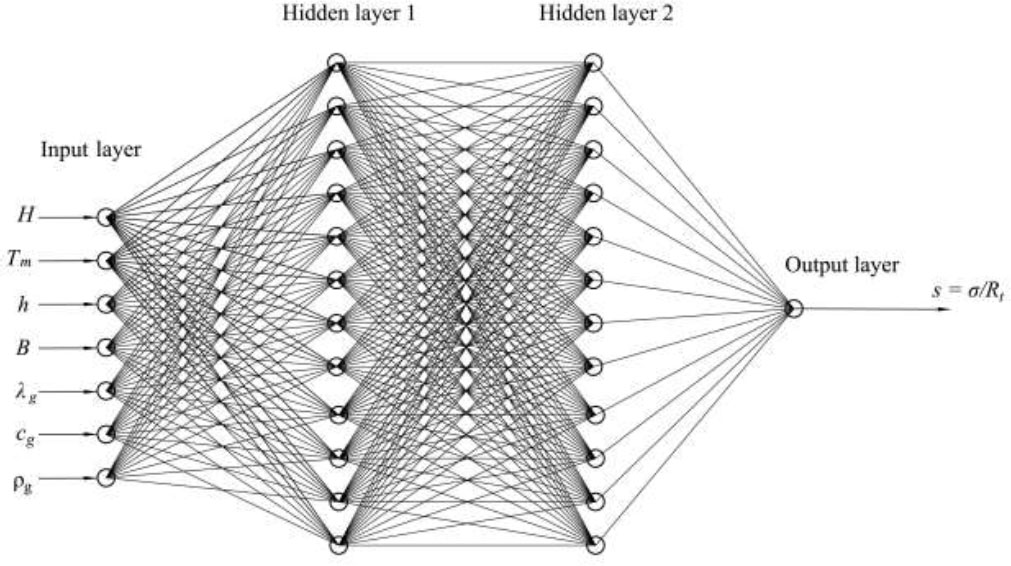
The architecture of artificial neural networks.
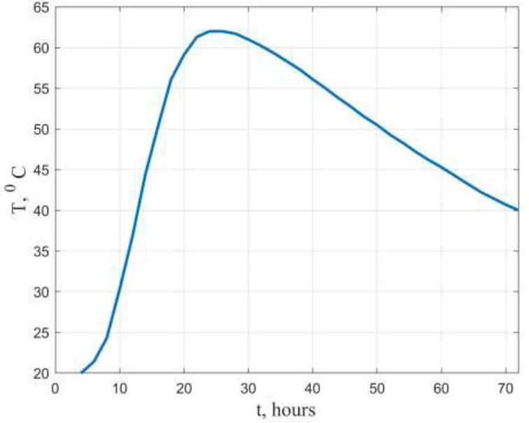
Temperature change over time for samples with 100% strain limitation.
The training dataset was standardly divided into three subsets: training, validation, and test. The split ratio was 75%:15%:15%. The division into subsets was performed randomly. The Mean Squared Error (MSE) value was chosen as a metric for the quality of training, which was calculated using the following formula (Eq 9):
 |
(9) |
Where n is the volume of the training dataset, Yi is the value of the stress level s predicted by the neural network, and Ti is the target value of the stress level S.
Minimization of the MSE value was performed using the Levenberg–Marquardt optimization algorithm. The number of iterations in the training process was fixed and equal to 1000.
3. RESULTS AND DISCUSSION
The theoretical model, on the basis of which the training dataset was formed, was preliminarily tested on the experimental data reported by previous studies [29, 30].
A study by Bjøntegaard Ø. [29] measured temperature stresses in hardening concrete samples with 100% strain limitation. The compressive strength of concrete at the design age of 28 days was R28 = 80 MPa. Fig. (2) shows the average graph of the change in temperature of the samples over time. Fig. (3) shows the change in temperature stress over time. The red line corresponds to the experimental values, and the blue line corresponds to the calculated values obtained using the formulas 3-5. These results can be considered satisfactory.
| Parameter | Value |
|---|---|
| Slab thickness H, m | 2.1 |
| Average ambient temperature Tm, °C | 17 |
| Heat transfer coefficient on the upper surface h, W/(m2∙°C) | 30 |
| Concrete grade B, MPa | 25 |
| Thermal conductivity coefficient of soil, λg W/(m∙°C) | 1.4 |
| Specific heat capacity of soil cg, J/kg∙°С | 2070 |
| Soil density ρg, kg/m3 | 1039 |
| Concrete hardening rate | Quick-hardening |
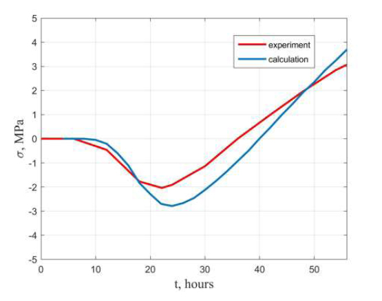
Graphs of stress changes over time for samples with 100% strain limitation.
Smolana et al. [30] presented the results of measuring temperature stresses in a hardening monolithic foundation slab located on a soil base. Table 3 presents the values of the quantities selected as input parameters of the ANN, with which the field experiment was conducted.
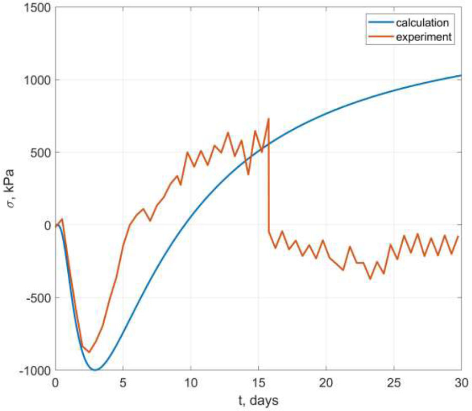
Comparison of experimental stresses in the foundation slab with calculated ones.
The stresses in the specified experiment were measured at z = H/2 (in the middle of the foundation slab thickness). Fig. (4) shows a comparison of the experimental stress values with the calculated ones. As shown in Fig. (4), the theoretical model, which was the basis for the formation of the training datasets, predicted stresses well at an age of up to 2.5 days. Furthermore, a deviation was observed, which may be caused by concrete shrinkage deformations, daily fluctuations in ambient temperature, features of the heat release kinetics of a specific concrete composition used in the experiment, etc. During the 16 days, an increase in stresses to almost zero was observed on the experimental graph, which is most likely associated with crack formation. At the moment of crack formation, the theoretical model quite accurately predicted the magnitude of tensile stress.
Table 4 presents a fragment of the generated training dataset with target values of stress level s for slow-hardening and quick-hardening concrete.
As presented in Table 4, in the case of using slow-hardening concrete, the stress level s was almost always higher than in the case of using quick-hardening concrete. However, this is true only for the selected fragment of the dataset. The minimum ratio s1 / s2, where s1 corresponds to the stress level for slow-hardening concrete, and s2 corresponds to the stress level for quick-hardening concrete, was 0.41. The maximum value of the ratio s1 / s2 was 2.36, and the average was 1.36. Thus, under some conditions, it is preferable to use slow-hardening concrete, and under other conditions, it is preferable to use quick-hardening concrete.
| No. | H, m |
Tm, °С |
h, W/(m2 ∙°С) |
B, MPa | λg, W/(m∙°С) |
cg, J/(kg∙°С) |
ρg, kg/m3 |
s | |
|---|---|---|---|---|---|---|---|---|---|
| Slow-hardening | Quick-hardening | ||||||||
| 1 | 0.7000 | 5 | 2 | 25 | 0.56 | 1500 | 1000 | 0.2283 | 0.2370 |
| 2 | 0.9875 | 5 | 2 | 25 | 0.56 | 1500 | 1000 | 0.3756 | 0.3408 |
| 3 | 1.2750 | 5 | 2 | 25 | 0.56 | 1500 | 1000 | 0.5294 | 0.4484 |
| 4 | 1.5625 | 5 | 2 | 25 | 0.56 | 1500 | 1000 | 0.6857 | 0.5611 |
| 5 | 1.8500 | 5 | 2 | 25 | 0.56 | 1500 | 1000 | 0.8418 | 0.6768 |
| 6 | 2.1375 | 5 | 2 | 25 | 0.56 | 1500 | 1000 | 0.9961 | 0.7939 |
| 7 | 2.4250 | 5 | 2 | 25 | 0.56 | 1500 | 1000 | 1.1473 | 0.9106 |
| 8 | 2.7125 | 5 | 2 | 25 | 0.56 | 1500 | 1000 | 1.2947 | 1.0256 |
| 9 | 3 | 5 | 2 | 25 | 0.56 | 1500 | 1000 | 1.4379 | 1.1381 |
| … | … | … | … | … | … | … | … | … | … |
| 759367 | 0.7000 | 35 | 30 | 45 | 2.67 | 2500 | 3500 | 1.0074 | 0.7368 |
| 759368 | 0.9875 | 35 | 30 | 45 | 2.67 | 2500 | 3500 | 1.4651 | 1.0760 |
| 759369 | 1.2750 | 35 | 30 | 45 | 2.67 | 2500 | 3500 | 1.8860 | 1.3773 |
| 759370 | 1.5625 | 35 | 30 | 45 | 2.67 | 2500 | 3500 | 2.2687 | 1.6397 |
| 759371 | 1.8500 | 35 | 30 | 45 | 2.67 | 2500 | 3500 | 2.6161 | 1.8674 |
| 759372 | 2.1375 | 35 | 30 | 45 | 2.67 | 2500 | 3500 | 2.9321 | 2.0662 |
| 759373 | 2.4250 | 35 | 30 | 45 | 2.67 | 2500 | 3500 | 3.2201 | 2.2415 |
| 759374 | 2.7125 | 35 | 30 | 45 | 2.67 | 2500 | 3500 | 3.4835 | 2.3973 |
| 759375 | 3.0000 | 35 | 30 | 45 | 2.67 | 2500 | 3500 | 3.7253 | 2.5368 |
Table 5.
| Parameter | Correlation Coefficient | |
|---|---|---|
| Slow-Hardening Concrete |
Quick-Hardening Concrete |
|
| Slab thickness | 0.8031 | 0.8269 |
| Average ambient temperature | 0.3282 | 0.1643 |
| Heat transfer coefficient on the upper surface | 0.3094 | 0.2854 |
| Concrete grade | 0.2405 | 0.3233 |
| Thermal conductivity coefficient of soil | -0.0995 | -0.1033 |
| Specific heat capacity of soil | -0.0324 | -0.0332 |
| Soil density | -0.0799 | -0.0818 |
Before training the models, a correlation analysis of the generated data was also carried out to preliminarily assess the significance of the input parameters. Table 5 presents the values of the correlation coefficient between the maximum value of the stress level s and the input parameters.
Table 5 indicates that there is a strong positive relationship between the stress level s and the slab thickness regardless of the concrete hardening rate, which is quite an obvious result. For slow-hardening concrete, there is a moderate positive relationship between the value s and the ambient temperature, as well as between s and the heat transfer coefficient on the upper surface. In the case of slow-hardening concrete, the relationship between the value s and the concrete grade is weakly positive. For quick-hardening concrete, on the contrary, the relationship between s and the concrete grade is moderately positive, and between s and Tm, as well as between s and h, the relationship is weakly positive.
The relationship between the thermal-physical characteristics of the soil (density, thermal conductivity, specific heat capacity) and the stress level s is weakly negative, regardless of the rate of concrete hardening.
Figs. (5 and 6) show the neural network training performance graphs for models 1 and 2, corresponding to slow-hardening and quick-hardening concrete. The lines corresponding to the training, validation, and test samples overlap each other, indicating that the volume of these samples is more than sufficient. Both models are characterized by MSE values close to zero.
Figs. (7 and 8) show the regression plots for models 1 and 2 for the training, validation, and test samples, as well as for the entire dataset. The abscissa axis of each graph shows the target values T of the stress level, and the ordinate axis shows the values Y predicted by the neural network. All points on these graphs are located on the straight line Y = T or near it. The correlation coefficients RYT between the target and predicted values are close to 1.
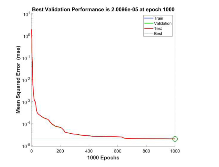
Neural network training performance graph for model 1 (slow-hardening concrete).
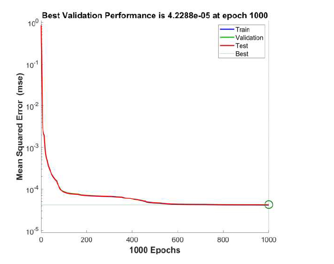
Neural network training performance graph for model 2 (quick-hardening concrete).
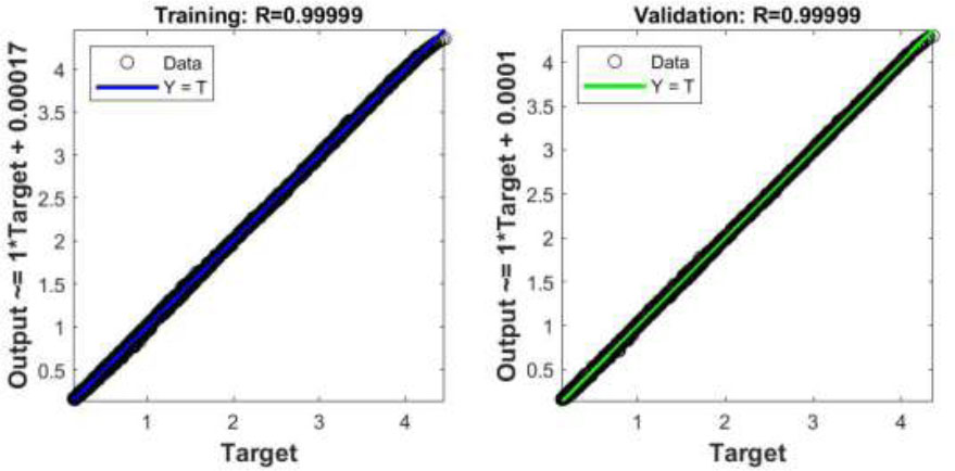
Regression plots for model 1 (slow-hardening concrete).
Artificial neural networks also allow us to evaluate the significance of features. The significance of the input parameters was evaluated using the method of fixing values. This method is based on the assumption that if a feature is redundant, then fixing its value at the corresponding input of the neural network will not lead to a noticeable change in the values at the output. The algorithm for determining the significance of features is as follows:
1. For the input parameter whose significance needed to be assessed, its average value in the training dataset was determined
 .
.
2. For each sample in the training dataset, the value of the objective function
 was determined when the input Xi was fixed.
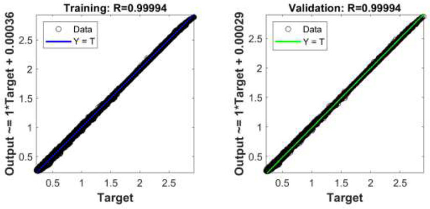
Regression plots for model 2 (quick-hardening concrete).
| Parameter | Significance of the Feature Zi | |
|---|---|---|
| Slow-Hardening Concrete |
Quick-Hardening Concrete |
|
| Slab thickness | 0.5459 | 0.4989 |
| Average ambient temperature | 0.1836 | 0.0839 |
| Heat transfer coefficient on the upper surface | 0.1614 | 0.1457 |
| Concrete grade | 0.1075 | 0.1343 |
| Thermal conductivity coefficient of soil | 0.0588 | 0.0517 |
| Specific heat capacity of soil | 0.0201 | 0.0176 |
| Soil density | 0.0472 | 0.0411 |
3. The significance of the feature for the current sample j was defined as the absolute relative difference between the value of the objective function s(w), characterizing the neural network with a full set of features, and the value
 (Eq 10):
 |
(10) |
4. The average value of the feature significance was determined for the entire training dataset (Eq 11):
 |
(11) |
Table 6 presents the significance values of the input parameters obtained using the method described above.
Table 6 presents that the most significant parameter influencing the risk of early cracking is the thickness of the foundation slab. Of interest is the fact that for slow-hardening concrete, the ambient temperature Tm has a greater effect on stress levels than it does for quick-hardening concrete.
The heat transfer coefficient on the upper surface has approximately the same effect on the stress level for both quick-hardening and slow-hardening concrete. Therefore, the main measure to prevent the risk of early cracking is to reduce the heat transfer coefficient on the upper surface by insulating it [31-33].
It is also quite interesting that the concrete grade influences the stress level s. On the one hand, with an increase in the concrete grade, its tensile strength Rt increases. On the other hand, the specific heat release also increases, and accordingly, the maximum value of tensile temperature stresses also increases. The increase in heat release with an increase in the concrete grade occurs faster than the increase in tensile strength. Therefore, with an increase in the concrete grade, an increase in the stress level is also observed.
The thermal properties of the soil base have a lesser influence on the stress level. This can be explained by the fact that, as a rule, most of the heat exchange occurs along the upper surface of the foundation slab.
CONCLUSION
In this study, two models of artificial neural networks were developed to predict the risk of early cracking during the construction of massive monolithic foundation slabs based on seven input parameters, including the thickness of the foundation slab, environmental and heat exchange conditions on the upper surface, concrete grade by compressive strength, and thermal properties of the soil base. The first model allowed for predicting the risk of early cracking for slow-hardening concrete, and the second model was used for quick-hardening concrete. These models were able to predict the early crack formation within the range of input parameters on which they were trained. The thickness of the foundation slabs could range from 0.7 to 3 m. The ambient temperature could vary from +5 to +35 °С, and the concrete grade could vary from B25 to B45 according to Russian standards. For the soil thermophysical characteristics and the heat transfer coefficient on the upper surface, all possible values were considered when generating the training dataset.
The constructed models are characterized by high forecast quality. The mean-square error of the forecast is close to zero, and the correlation coefficients between the target and predicted stress level values are close to 1.
Furthermore, the significance of the models' input parameters was assessed using the value fixation method. It was found that the most significant parameter affecting the risk of early cracking is the thickness of the foundation slab. It was found that for slow-hardening concrete, the average ambient temperature has a greater effect on the stress level than for quick-hardening concrete. One of the most significant parameters is the heat transfer coefficient on the upper surface of the slab. It was found that the concrete grade has an effect on the stress level. The thermophysical characteristics of the soil base have virtually no effect on the risk of early cracking.
It should be noted that previously, experimental studies were only conducted on the influence of the foundation slab thickness and the heat transfer coefficient for the upper surface on the risk of early crack formation. However, the influence of heat exchange conditions at the boundary between the foundation slab and the soil base has not been previously experimentally studied. In the future, we plan to conduct such a study to confirm the obtained theoretical results.
In this study, concrete shrinkage was not taken into account when training artificial intelligence models since its value can vary significantly depending on the composition of the concrete. Our further research will also be aimed at developing machine-learning models that take this factor into account.
AUTHORS’ CONTRIBUTION
It is hereby acknowledged that all authors have accepted responsibility for the manuscript's content and consented to its submission. They have meticulously reviewed all results and unanimously approved the final version of the manuscript.
LIST OF ABBREVIATIONS
| ANN | = Artificial Neural Networks |
| RF | = Random Forest |
| CNN | = Convolutional Neural Network |

