All published articles of this journal are available on ScienceDirect.

Excess Pore Water Pressure Ratio Comparison from Empirical and Numerical Methods to Determine Liquefaction Potential in Palu, Central Sulawesi, Indonesia
Abstract
Background
Palu is a city in Central Sulawesi Province with a very high level of seismic activity. The seismicity in Central Sulawesi is associated with the active movement of the Palu Koro fault. One of the most severe events occurred on September 28, 2018, which triggered liquefaction and a tsunami. This is also related to the lithology of Palu, which consists of alluvial deposits predominantly made up of sand.
Objective
This study compares excess pore water pressure values analyzed empirically and numerically to identify liquefaction potential. It aims to provide additional perspectives for engineers in designing buildings around the study area that are resistant to liquefaction.
Methods
Excess pore water pressure was analyzed using empirical and numerical methods to determine liquefaction potential. The empirical method used the equation by Yegian and Vitteli (1981), while the numerical method involved finite element analysis using the Plaxis 2D application and nonlinear analysis using DEEPSOIL v7.
Results
The results from the three methods of analyzing excess pore water pressure to determine liquefaction potential at the four borehole points showed differences. For the empirical method, using the equation by Yegian and Vitelli (1981), the results indicated that the layers with a pore pressure ratio (ru>0.8) were deeper than the finite element and non-linear methods.
Conclusion
The differences in methods result in varying outcomes in analyzing excess pore water pressure to identify liquefaction potential. The empirical method uses the peak value of Peak Ground Acceleration (PGA) to evaluate the entire soil profile, leading to a more generalized assessment. In contrast, the non-linear and finite element methods consider each layer's behavior under the applied seismic load, providing more detailed and similar results.
1. INTRODUCTION
Palu is located in an area of high seismicity, especially due to its location along the Palu Koro fault line. This fault is one of the most active faults in Indonesia and is prone to earthquakes. The Palu Koro fault extends from Central Sulawesi to the Moluccas Sea, and the area it crosses, including the city of Palu, is prone to earthquakes due to active fault movement.
The earthquake that struck the city of Palu on September 28, 2018, triggered a tsunami and liquefaction disaster. A total of 2,200 people were reported dead, with 1,000 missing and 4,500 injured [1]. This disaster is the largest in the history of Palu City.
Liquefaction is a phenomenon where sandy soil experiences shocks that cause a sudden increase in pore water pressure, causing the loss of bonds between soil particles. As a result of the loss of these bonds, the soil loses its strength and stiffness, so it cannot support the load of the structure built on it.
The level of liquefaction susceptibility is important in planning a building in areas with sandy soil and high seismic activity. This factor influences the design of foundations suitable for supporting the building during liquefaction.
According to Indonesia's Liquefaction Susceptibility Zone, Palu City has a very high liquefaction potential [2]. This is due to the city's soil lithology, which consists of alluvial and coastal deposits with materials such as sand, silt, and coral [3]. In addition to its sand-dominated lithology, Palu City experiences very high seismic activity, further contributing to its high liquefaction potential.
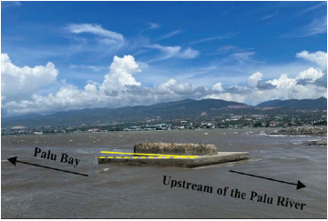
Pile cap on the pier of the old bridge that has collapsed.
The calculation of liquefaction analysis is supported by the discovery of liquefaction phenomena in the study area. In the research conducted by Sassa and Takagawa in 2018 [4], characteristics indicating that the study area experienced liquefaction were found, including sand boils around the bridge structures. During the study, other phenomena were also observed, such as changes in the inclination of the pile cap on the old bridge pier, which collapsed during the 2018 event, as demonstrated in Fig. (1). Additionally, it was found that the foundation of the retaining wall near the study location experienced deformation, as illustrated in Fig. (2).
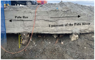
Foundation structure of the retaining wall on the palu river.
Research on liquefaction potential analysis has been extensively conducted. Generally, liquefaction potential analysis uses the Standard Penetration Test (SPT) parameter, with the output being a comparison between the Cyclic Resistance Ratio (CRR) and the Cyclic Stress Ratio (CSR) [5]. CRR refers to the cyclic resistance ratio of the soil to withstand shear stress during an earthquake, while CSR represents the shear stress caused by the earthquake that could lead to soil liquefaction.
The study site is located on the eastern bank of the downstream Palu River. Research related to liquefaction risk based on excess pore water pressure ratio values at the study site has never been conducted, making it an interesting subject for investigation. Similar studies were performed on the Balaroa area, with a potential liquefaction level reaching 9 m, the Petobo area, with a 6–10 m depth, and the Jono Oge area, with a potential liquefaction depth reaching 17 m [6].
This study analyzes liquefaction potential by comparing the excess pore water pressure values obtained from empirical calculations and numerical calculations using the Plaxis 2D and DEEPSOIL v7 applications. The Peak Ground Acceleration (PGA) parameter refers to the 2017 Earthquake Hazard and Source Map, with a 7% probability of exceedance in 75 years [7].
2. MATERIALS AND METHODS
2.1. The Research Area
The research area is located downstream of the river in the eastern part of Palu City. This study is based on four soil investigation borehole points, BH 1, BH 2, BH 3, and BH 4, as shown in Fig. (3). The Palu 4 Bridge is being constructed in the research area, specifically on the eastern side abutment and embankment.
2.2. Geological and Geotechnical Condition
The research location consists of alluvial and coastal deposits. Its position downstream of the Palu River results in sediment transport quite far from the weathering source, leading to sand grains with rounded shapes. The rounded grain shape reduces the interlocking between particles. Additionally, these deposits formed during the Quaternary period, meaning the sediments' cementation process has not yet occurred [8].
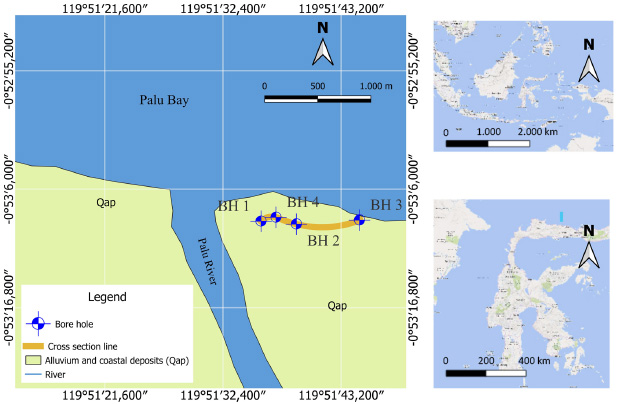
Borehole location in the research area [3].
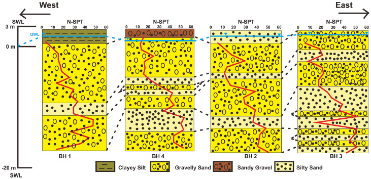
The cross-sectional profile of soil layers extending from west to east.
Palu City is located along the Palu Koro Fault, a strike-slip fault that moves at a rate of 42 mm per year [9]. This movement is associated with the high seismic activity in the area. The research location is at the mouth of the Palu River, which is directly connected to Palu Bay, resulting in a shallow groundwater table. With sandy soil, high seismic activity, and a shallow groundwater level, there are early indications that the research location is prone to liquefaction.
Based on the sieve analysis results, the lithology of the four borehole points indicates that the lithology consists of clayey silt and sandy gravel up to a depth of 20 meters. The NSPT values at the four borehole points vary, ranging from 6 to 50, as shown in Fig. (4). The four borehole points have different groundwater levels: BH 1 has a groundwater depth of 1.1 m with a drilling elevation of 2.72 m above sea level, BH 2 has a depth of 1.05 m with a drilling elevation of 2.52 m above sea level, BH 3 has a depth of 0.6 m with a drilling elevation of 2.54 m above sea level, and BH 4 has a depth of 1.74 m with a drilling elevation of 3.08 m above sea level.
2.3. Data Acquisition
The data consists of soil investigation data from Standard Penetration Test (SPT) values from four boreholes: BH 1, BH 2, BH 3, and BH 4. This study also utilizes laboratory test data.
The ground motion data used are earthquake recordings from the Pacific Earthquake Engineering Research Center (PEER) via the website https://ngawest2. berkeley.edu/, with input parameters derived from deaggregation using the Indonesian Earthquake Hazard Deaggregation Map for Seismic-Resistant Infrastructure Planning and Evaluation [10]. Once determined, the ground motion matches the target design spectra created based on the Indonesian National Standard 2833:2016 [11].
2.4. Data Analysis
The field measurement data from the Standard Penetration Test (SPT) is corrected using several correction factors, such as overburden pressure correction, correction for the energy ratio produced by the hammer blow, borehole diameter correction, SPT rod length correction, fine grain content correction, and correction for the liner of the SPT sampler [12].
After applying the corrections to the SPT values, the next step is calculating the Cyclic Resistance Ratio (CRR) with a correction factor for effective overburden pressure correction (Kσ). The earthquake magnitude used is 7.5 Mw, referring to the Palu earthquake that occurred on September 28, 2018. The CRR value is calculated using Eq. (1) mentioned below [13].
 |
(1) |
where CRRM,σ'v represents the CRR value that has been corrected with the magnitude scaling factor (MSF) and the effective overburden pressure correction (Kσ).
The factor of safety against liquefaction requires the analysis of the Cyclic Stress Ratio (CSR) using Eq. (2). The CSR is calculated using the Peak Ground Acceleration (PGA) value of 0.794g from the Indonesian Seismic Code, with a 7% probability of exceedance over 75 years. The total vertical stress influences the CSR value (σv), effective vertical stress (σ'v), maximum ground acceleration due to the earthquake, gravitational acceleration (g), and the stress reduction factor (rd). The equation is as follows:
 |
(2) |
The Safety Factor (SF) value is the ratio between the CRR and CSR values, as shown in Eq. (3) below.:
 |
(3) |
The Boulanger and Idriss (2014) method is commonly used for identifying liquefaction potential. This method can be applied using data that are typically available, such as N-SPT values, as well as laboratory test data commonly performed, such as specific gravity, plasticity index for silt and clay, and sieve analysis. Therefore, the Simplified Procedures method is the most suitable empirical method for this research.
The obtained safety factor results are then processed using the equation given by Yegian and Vittelli in 1981 [14] to determine the excess pore water pressure ratio (ru), as shown in Eq. (4) below, where α and β values are 0.7 and 0.19, respectively.
 |
(4) |
The Yegian and Vittelli (1981) method presents the results of the simplified procedure calculations from Boulanger and Idriss (2014), which are expressed as the excess pore water pressure ratio (ru) to facilitate comparison with the nonlinear and finite element methods. These comparison results will be part of the analysis in this study. Although this method was introduced many years ago, it is still widely used by several recent authors [15-17].
The target spectra are determined using the PGA value, the spectral value at the ground surface for a 1-second period (SDS), and the spectral value at the ground surface for a short period of 0.2 seconds (SD1). The value of SDS is obtained from https://lini.binamarga.pu.go.id/ based on reference [9]. Several parameters are needed to establish the target spectra to define the curve boundaries. The first parameter required is the initial transition period from the phase of maximum acceleration (T 0), followed by the transition period where spectral acceleration starts to decrease as the period increases (TS). After the period TS, the spectral acceleration (Sa) is determined. These parameters can be calculated using Eqs. (5-7), given as follows:
 |
(5) |
 |
(6) |
 |
(7) |
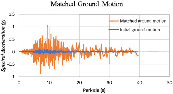
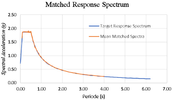
After determining the target spectrum, matching is performed so that the ground motion can be adjusted to field conditions. The matching results are shown in Fig. (5). The results of the ground motion matching that has been performed can be seen in Fig. (6).
2.5. Nonlinear Site Response Analysis
Numerical analysis is conducted as a comparison to the empirical method [14, 15]. Numerical analysis can be performed using 1-D Site Specific Response Analysis (SSRA) with the DEEPSOIL v7 application to estimate the excess pore water pressure. This analysis uses the Generalized Quadratic/Hyperbolic (GQ/H+PWP) approach.
The main parameters for numerical analysis using DEEPSOIL v7 with the Dorby and Matasovic Model Parameters for sand layers are normalized excess pore pressure (UN), equivalent number of cycles (>Neq), current reversal shear strain (>γc), threshold shear strain value (>γtvp), curve fitting parameters (P, s, and F), dimensionality factor (f), and degradation parameter (v).
Comparison of target response spectrum and matched response spectrum results.
Comparison of initial ground motion and matched ground motion results.
In its calculations, this model is influenced by the Fines Content (FC) and shear wave Velocity (VS) values [18], as shown in Eqs. (8 and 9) below:
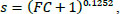 |
(8) |
 |
(9) |
The parameter v is calculated using Eq. (10) given below, where Dr represents the relative density in %.
 |
(10) |
For clay layers, the Matasovic and Vucetic (1995) model parameters are used, with key parameters including normalized excess pore pressure (UN), equivalent number of cycles (Neq), current reversal shear strain (γC), threshold shear strain value (γtvp), curve fitting parameters (r and s), and curve fitting coefficients (A, B, C, and D). The values for each parameter are based on Matasovic and Vucetic (1995) for marine clay material (OCR 1.0).
The ru analysis using the nonlinear method is performed to account for the nonlinear behavior of the soil during an earthquake. The PGA value, which is one of the triggers of liquefaction, will be adjusted according to the soil response. This method is used to determine the amplification of earthquake vibrations, which in turn increases pore water pressure, leading to liquefaction.
2.6. Finite Element Method
Excess pore water pressure can be calculated numerically using the Plaxis 2D application with the PM4Sand model. Plaxis 2D utilizes the finite element method to analyze and estimate the increase in pore water pressure. PM4Sand simulates the behavior of sand under dynamic conditions, which generates the values of pore water pressure increase, liquefaction conditions, and displacement values following the dynamic event [19].
The main parameters in the PM4Sand model are atmospheric pressure (pA), contraction rate parameter (hpo), shear modulus (G 0), and relative density (DR) [20]. The atmospheric pressure value used is 101.3 kPa.
The relative density (DR) parameter is obtained using the equation from Idriss and Boulanger (2008) [21], with parameters including the corrected SPT value at 1 atm overburden ((N1)(60) and other values as shown in Eq. (11) below:
 |
(11) |
Shear modulus coefficient (G0) controls the small strain shear (elastic), the expression covering a range of typical densities can be used to calculate the parameter directly G0 as proposed by Boulanger and Ziotopoulou (2015) [22] in Eq. (12) given below:
 |
(12) |
The steps to obtain the contraction rate parameter require using the Cyclic Direct Simple Shear (CDSS) test. This is conductedto calibrate the CRR value under cyclic conditions. Liquefaction is considered to occur when the peak shear strain reaches 3% after undergoing cycles in the CDSS test.
| Parameter | Value | Unit |
|---|---|---|
| α | 0.096 | - |
| β | 0.00079 | - |
| e | Laboratory data | - |
| DR | Eqs.5 | - |
| G 0 | Eqs.6 | - |
| hp0 | CDSS testing | - |
| pA | 101.3 | kPa |
| emax | 0.8 | - |
| emin | 0.5 | - |
| nb | 0.5 | - |
| nd | 0.1 | - |
| φCV | 33 | o |
| Q | 10 | - |
| R | 1.5 | - |
The input parameters for the sand layer analysis using the PM4Sand model include unsaturated unit weight (γunsat), saturated unit weight (γsat), void ratio (einit), Rayleigh damping with a value of 0.096 for Rayleigh α and 0.00079 for Rayleigh β, initial relative density (DR), shear modulus coefficient (G 0), contraction rate (hp0), atmospheric pressure (pA), maximum void ratio (emax), minimum void ratio (emin), bounding surface position according to ξR(nb), bounding surface position according to ξξR(nd), critical state friction angle (φCV), critical state line parameters for Q and R, and the earth pressure coefficient K 0, with each value as shown in Table 1.
| Parameter | Value | Unit |
|---|---|---|
| α | 0.096 | - |
| β | 0.00079 | - |

|
9,000 | kN/m2 |

|
9,000 | kN/m2 |

|
27,000 | kN/m2 |
| m | 1 | - |
| cref' | 30 | kN/m2 |
| φ' | 26 | o |
| ψ | 0 | o |
| γ0.7 | 0.0007 | - |

|
60,000 | kN/m2 |
| vur' | 0.2 | - |
| Pref | 100 | kN/m2 |

|
0.5616 | - |
| cinc' | 0 | kN/m2/m |
| yref | 0 | m |
| Rf | 0.9 | - |
| OCR | 2 | - |
The parameters used for the clay layer utilize the HS small model. This model includes several input parameters such as secant stiffness in standard drained triaxial test
 tangent stiffness for primary oedometer loading
 power for the stress-level dependency of stiffness (m), cohesion
 friction angle (φ'), unloading/reloading stiffness
 dilatancy angle (ψ), shear strain at which Gs = 0.722 G0 (γ0.7) shear modulus at very small strains
 Poisson's ratio
 reference stress (Pref), cohesion increment (cinc'), reference coordinate (yref), failure ratio (Rf), and Over Consolidation Ratio (OCR), as demonstrated in Table 2.
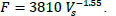
Safety factor values for 4 borehole points.
The analysis of ru using the finite element method with the help of Plaxis 2D is employed to provide a more detailed simulation of the pore water pressure ratio increase during an earthquake. The finite element method divides the entire soil layers into smaller elements, allowing for more precise and accurate analysis.
This study is conducted in stages, starting with an analysis using an empirical method that simplifies the calculation process. Next, a non-linear method is applied to analyze each soil layer individually, providing a more detailed soil response compared to the empirical method. Finally, the finite element method is used to divide the entire soil layers into smaller elements, yielding more detailed and accurate results.
3. RESULTS AND DISCUSSION
3.1. Liquefaction Potential Analysis using the Empirical Method
Liquefaction potential analysis at four borehole points was conducted using the simplified procedure introduced by Boulanger and Idriss (2014) [13]. The earthquake parameter used in the study was a magnitude of 7.5 Mw, which occurred in Palu City on September 28, 2018, with a PGA value of 0.794g. Liquefaction is unlikely to occur at depths greater than 20 meters [23]. A study by Iwasaki in 1981 on the liquefaction potential index also limits liquefaction potential to a depth of 20 meters [24]. Based on previous research, empirical analysis was conducted up to a depth of 20 meters.
The results of soil data processing using the simplified procedure by Boulanger and Idriss (2014) [13] indicate that borehole BH 1 has liquefaction potential up to a depth of 17 m, borehole BH 2 up to a depth of 12 m, borehole BH 3 up to a depth of 15 m, and borehole BH 4 up to a depth of 13.5 m, as shown in Fig. (7).
Excess pore water pressure calculation using the Yegian and Vitelli (1981) equation employs parameters such as the liquefaction safety factor value. Thus, for layers with liquefaction potential, the limit with an ru value > 0.8 is at the same depth as the SF value < 1, as shown in Fig. (8).
3.2. Liquefaction Potential Analysis Using Numerical Methods
In conducting liquefaction risk analysis using numerical methods, ground motion is required as the earthquake load to observe the soil's response to seismic loading. This study used ground motion from the Imperial Valley earthquake in 1979, with a magnitude of 6.5 Mw and a strike-slip fault mechanism. This ground motion is then matched to the target spectrum to approximate the ground motion conditions at the research location.
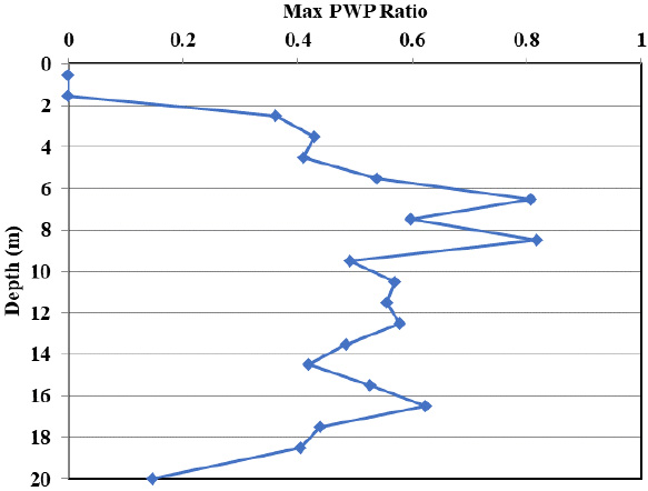
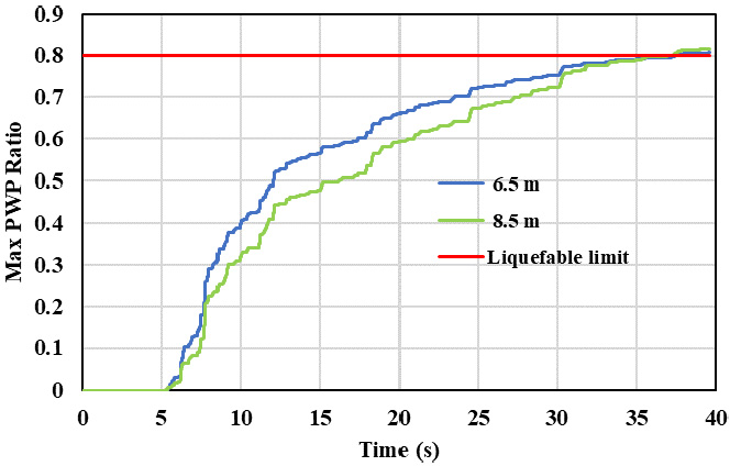
At point BH 1, data processing using DEEPSOIL v7 shows that layers with an ru > 0.8 are located at depths of 6.5 m and 8.5 m, as shown in Fig. (9). The results also indicate an increase in Pore Water Pressure (PWP) ratio at 37.4 seconds for the 6.5 m layer and 37.2 seconds for the 8.5 m depth layer, as shown in Fig. (10). The liquefied layer is a gravelly sand layer with an average N-SPT value of 14 and 17.
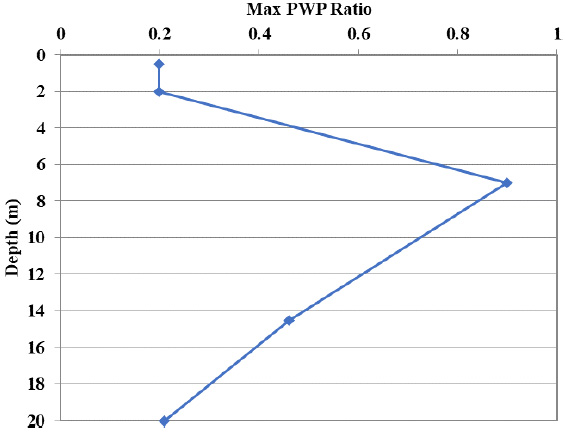
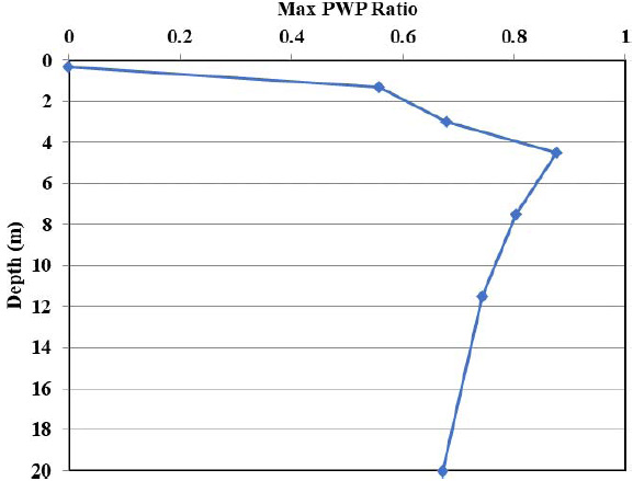
At point BH 2, data processing with DEEPSOIL v7 shows an ru > 0.8 at a depth of 7 m, as shown in Fig. (11). The results also indicate that ru > 0.8 occurs at 21.6 seconds, as shown in Fig. (12). The liquefied layer is a silty sand to gravelly sand layer with an average N-SPT value of 14 and 17.
At point BH 3, data processing using DEEPSOIL v7 shows an ru value > 0.8 at depths of 4.5 m and 7.5 m, as shown in Fig. (13). The results also indicate an increase in ru > 0.8 at 20.8 seconds for the soil layer at a depth of 4.5 m and at 37.2 seconds for the soil layer at a depth of 7.5 m, as shown in Fig. (14). The liquefied layer is a silty sand to gravelly sand layer with average N-SPT values of 9 and 20.
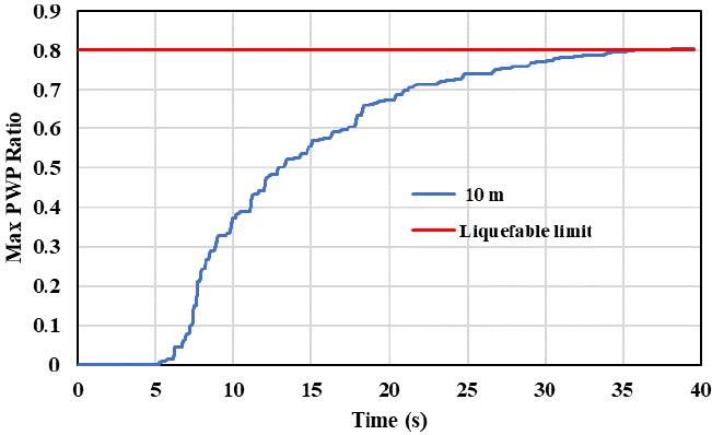
At point BH 4, data processing with DEEPSOIL v7 shows an ru > 0.8 at a depth of 10 m, as shown in Fig. (15). The results also indicate that ru > 0.8 occurs at 35.7 seconds, as shown in Fig. (16). The liquefied layer is a gravelly sand layer with an average N-SPT value of 17.
The analysis results of the increase in pore water pressure ratio (ru) using the nonlinear method show that liquefaction occurs in the silty sand to gravelly sand layers with an N-SPT range of 9 to 20. In the time history analysis, liquefaction begins after 21 seconds.
A numerical analysis was conducted using another tool, Plaxis 2D, with the PM4Sand model to compare the numerical method. The results show that borehole GA 04 has an ru > 0.8 at 2-9 m depth, as shown in Fig. (17). The liquefied layer is a gravelly sand layer with an average N-SPT value of 9 and 17.
At borehole BH 2, liquefaction occurred down to a depth of 11 m. This is indicated by an ru value greater than 0.8 at 3 m and 11 m depths, as demonstrated in Fig. (18). The liquefied layer consists of silty sand and gravelly sand layers with average N-SPT values of 6 and 17.
At borehole BH 3, liquefaction occurred down to a depth of 10 m. This is indicated by an ru value greater than 0.8 at depths of 0-2 m, followed by depths of 4-5 m and 5-10 m, as shown in Fig. (19). The liquefied layer consists of silty sand and gravelly sand layers with average N-SPT values ranging from 6 to 20.
At borehole, BH 4, the Plaxis 2D calculations indicate a liquefied layer at a depth of 6.25 m. This is shown by an ru value greater than 0.8 at a depth of 6.25 m, as illustrated in Fig. (20). The liquefied layer consists of gravelly sand with an average N-SPT value of 17.
The results obtained from the finite element method analysis indicate that the liquefied layer consists of silty sand to gravelly sand with N-SPT values ranging from 6 to 20. An interesting finding from the finite element method is that when a layer has a significant potential for liquefaction, with a thickness greater than the critical threshold, the ru value exceeding 0.8 is not evenly distributed throughout the entire layer. Instead, the high ru values are concentrated at the lower boundary of the layer.
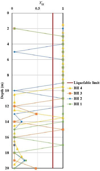
ru values for 4 borehole points using the Yegian and Vitelli (1981) method.
| Borehole | Yegian and Vitelli (1981) | DEEPSOIL v7 | Plaxis 2D |
|---|---|---|---|
| BH 1 | 17 m | 8.5 m | 9 m |
| BH 2 | 12 m | 11 m | 11 m |
| BH 3 | 15 m | 10 m | 10 m |
| BH 4 | 13.5 m | 13.95 m | 6.25 m |
ru value at borehole BH 1.
Time history of ru at borehole BH 1.
ru value at borehole BH 2.
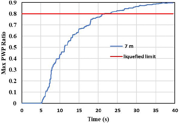
Time history of ru at borehole BH 2.
ru value at borehole BH 3.
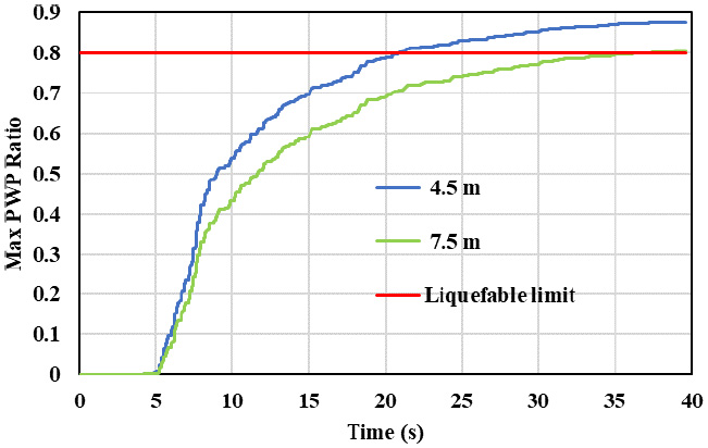
Time history of ru at borehole BH 3.
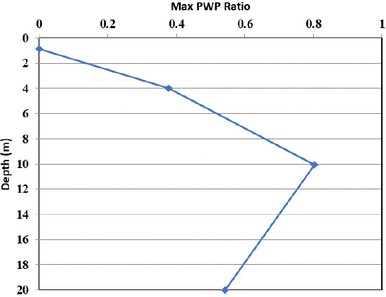
ru value at borehole BH 4.
Time history of ru at borehole BH 4.
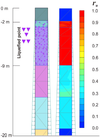
Liquefied point at borehole BH 1.
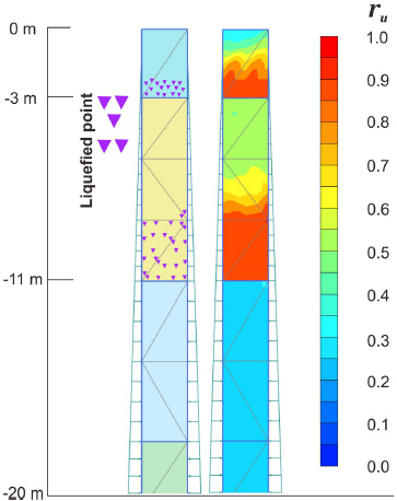
Liquefied point at borehole BH 2.
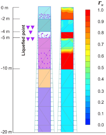
Liquefied point at borehole BH 3.
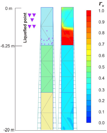
Liquefied point at borehole BH 4.
CONCLUSION
The study area is located near the Palu Koro fault line, which is actively moving and results in relatively high earthquake intensity. The shallow groundwater table combined with the unconsolidated sandy lithology in the area makes the study location highly susceptible to the risk of liquefaction.
This study used the earthquake parameters of the Palu earthquake on September 28, 2018, with a magnitude of 7.5 Mw and a PGA value of 0.794g, according to the 2017 earthquake hazard map. For the ground motion input in numerical calculations, the Imperial Valley-06 ground motion was used, sourced from the database at https://ngawest2.berkeley.edu/. This ground motion was then matched to align with the site conditions.
The liquefaction analysis was conducted at 4 borehole points using the simplified procedure: BH 1, BH 2, BH 3, and BH 4. At all four boreholes, liquefaction potential was identified at varying depths: for BH 1 at a depth of 17 m, for BH 2 down to 12 m, for BH 3 down to 15 m, and for BH 4 down to 13.5 m. After determining the safety factor against liquefaction potential at each borehole, the pore water pressure increase was calculated using the empirical method by Yegian and Vittelli (1981). In this method, excess pore water pressure values greater than 0.8 indicate the onset of liquefaction. The calculation results demonstrated that the layers with increased pore water pressure exceeding 0.8 matched those experiencing liquefaction, as the calculation parameters were based on the liquefaction safety factor.
The calculation of excess pore water pressure was also conducted using numerical methods with the help of DEEPSOIL v7 and Plaxis 2D software. According to the results from DEEPSOIL v7, for BH 1, layers with a pore pressure ratio (ru >0.8) were found at depths of 8.5 m and 6.5 m; for BH 2, at depths of 3-11 m; for BH 3, at depths of 4-10 m; and for BH 4, at depths of 6.25-13.95 m, as shown in Table 3.
Calculations using Plaxis 2D were performed for comparison. The results showed that for BH 1, layers with a pore pressure ratio (ru > 0.8) were found at a maximum depth of 9 m; for BH 2, at a maximum depth of 11 m; for BH 3, the deepest layer with ru > 0.8 was at 10 m, and for BH 4, liquefaction occurred down to a depth of 6.25 m, as detailed in Table 3.
Several interesting findings in this study show that the analysis using the nonlinear method with the DEEPSOIL v7 application produces a single result for each layer. If that layer is liquefied, the entire layer is considered liquefied, regardless of its thickness. In contrast, the analysis using the finite element method with the Plaxis 2D application can yield different values for a single layer. This indicates that the finite element method performs a more detailed analysis and limits the ru values according to its critical threshold.
There are significant differences in the calculation of excess pore water pressure. The results of ru calculations using the empirical method indicate that layers experiencing an increase in pore water pressure greater than 0.8 are deeper than the results produced by the non-linear and finite element methods. This discrepancy is related to the use of PGA values: the empirical method uses the peak PGA value for analyzing each layer independently, while the non-linear and finite element calculations adjust the PGA value according to soil conditions and account for the interactions between layers.
The results of this study can be applied to construction projects in areas with similar lithological conditions and groundwater table depths as the study area. Given the potential for soil liquefaction, mitigation measures are essential for any nearby development. It is crucial to anticipate axial bearing capacity issues due to possible negative skin friction and lateral bearing capacity concerns due to potential deformation beyond acceptable limits. These considerations are necessary to ensure the infrastructure built is resilient to liquefaction risks.
AUTHORS’ CONTRIBUTION
It is hereby acknowledged that all authors have accepted responsibility for the manuscript's content and consented to its submission. They have meticulously reviewed all results and unanimously approved the final version of the manuscript.
LIST OF ABBREVIATIONS
| CDSS | = Cyclic Direct Simple Shear |
| CRR | = Cyclic Resistance Ratio |
| CSR | = Cyclic Stress Ratio |
| SPT | = Standard Penetration Test |
| PEER | = Pacific Earthquake Engineering Research Center |
| MSF | = Magnitude Scaling Factor |
| PGA | = Peak Ground Acceleration |
AVAILABILITY OF DATA AND MATERIALS
The data and supportive information are available within the article.
FUNDING
This work was financially supported by Ministry of Public Works and Housing of Indonesia, Indonesia (Grant number 21310/UN1/FTK/DTSL/ HK.08.00/2023).
ACKNOWLEDGEMENTS
We extend our gratitude to the National Road Implementation Agency (BPJN) of Central Sulawesi Province, particularly to the Working Unit of National Road Implementation (PJN) Region I, for their support in providing data for this research.