All published articles of this journal are available on ScienceDirect.

Artificial Neural Network Models for Predicting Required Cross-section Dimensions of Concrete Filled Steel Tubular Columns
Authors Info & Affiliations
Abstract
Background
Artificial Neural Networks (ANN) can be a useful tool to assist in the design of reinforced concrete structures. The aim of this paper is to develop artificial neural network models for predicting the required diameter of eccentrically compressed concrete-filled steel tubular (CFST) columns and the wall thickness of the steel pipe.
Methods
Within the framework of the set goal, three models of ANN were developed. The first model predicts the required cross-sectional diameter for the minimum pipe wall thickness. The second model solves the same problem for the maximum possible wall thickness. The input parameters of the first two models are the axial force, bending moment, strength characteristics of steel and concrete, column length, and a coefficient characterizing the share of constant and long-term loads in the total load. The third model predicts the required wall thickness based on the listed parameters, as well as the column diameter. Synthetic data, including more than 2 million samples, was generated to train the models. The ANN architecture is a feedforward neural network with 2 hidden layers containing 16 neurons each. Machine learning models are implemented in the MATLAB environment.
Results
The trained models showed high performance in terms of mean squared error and correlation coefficient between the target and predicted values of the output parameter. The importance of features was also assessed using the variable fixation method. It has been established that the required value of the column diameter is most significantly influenced by the magnitude of the bending moment, axial force and column length. The required pipe wall thickness is most influenced by the magnitude of internal forces and the diameter of the column.
Conclusion
The developed models of artificial neural networks are an effective and reliable tool that can help a civil engineer in the design of buildings and structures that include CFST elements.
1. INTRODUCTION
In conditions of limited urban space, modern construction tends to increase the height of buildings and floor spans, which dictates the need to use columns with high load-bearing capacity. One of the promising solutions to this problem is concrete-filled steel tubular (CFST) structures, which provide an optimal combination of strength and functionality. Circular CFST columns have high axial compressive strength [1], which is their main advantage and allows them to be widely used in modern construction, including high-rise buildings, long-span bridges, underground tunnels and unique infrastructure facilities [2-4].
The ability to maintain structural integrity and stability in emergency situations is of key importance for CFST structures due to the ability to effectively absorb significant amounts of energy during deformation [5, 6]. In addition, such structures help reduce the impact on the environment due to the rejection of the traditional formwork use, recycling of steel pipes and the use of high-quality concrete with recycled aggregate [7].
Research conducted in the field of improving the calculation of CFST columns can be divided into several categories: full-scale experiments, calculations performed in accordance with national design standards (Eurocode4, AISC 360-16, SR 266.1325800.2016, etc.), numerical calculations in finite element software packages (ABAQUS, ANSYS, etc.) [8], artificial intelligence (AI) technologies and research that combine the above methods.
Laboratory experimental studies have traditionally been used to analyze the behavior of CFST columns, but their application is limited by a narrow parameter range, high cost, and significant labor costs. Kloppel and Gorder [9] conducted the first experimental studies of CFST columns in the 1950s. Since then, many experimental studies have been conducted to analyze the structural behavior of CFST columns [10-15]. The geometric and physical-mechanical data obtained from these and other experimental studies are actively used to train and test artificial intelligence models aimed at predicting the design results of CFST columns. AI models provide a better fit to experimental data and increased adaptability, overcoming the limitations of traditional nonlinear or analytical models [16].
Over the past 10 years, there has been an exponential growth in publications on CFST calculation using machine learning (ML) technologies. It can be confirmed by a search carried out in the Google Scholar scientometric database by keywords “CFST” and “ Machine Learning.”
Numerous studies have demonstrated the effectiveness of ANNs (artificial neural networks) technology in solving complex problems in the field of CFST calculation.
Thus, the authors of papers [17, 18] investigated the prediction of the bearing capacity for short CFST columns under axial load using ANN based on a large amount of experimental data. Comparative analysis of ANN and the empirical regression model revealed a clear advantage of ANN. R2 (the coefficient of determination) was 0.97 for ANN versus 0.926 for the regression model, and MAPE (mean absolute percentage error) reached 5.8% for ANN and 13.2% for the regression model. The study demonstrated that the use of ANN allows for achieving greater accuracy in predicting the bearing capacity of CFST columns compared to the previously proposed empirical regression model. Du et al. [19]. also used ANN technology for rectangular columns with good results. The mean value of output parameters μ was equal to 1.013, which shows a small deviation from the expected value. The coefficient of variation CoV was equal to 0.0702, which indicates good stability of the model. These metrics indicate that the neural network model has stable predictions with a small deviation from the mean.
Le et al. [20]. used Gaussian process regression (GPR) to predict the ultimate bearing capacity of rectangular CFST columns. As shown in this study, this method provides high prediction accuracy for the following metrics: R2 = 0.9956, RMSE = 154.66 (root mean square error), MAPE = 7.54%, the values of which indicate high agreement between the predicted and experimental values.
Tran’s works [21-23] present approaches to predicting the strength of columns using ANN models and a polynomial regression model. In a study [23], ANN demonstrated high prediction accuracy: μ=1.05, CoV =0.07, R2 = 0.996, a20-index = 0.993 (accuracy index) and MSE = 0.011535. These indicators confirm the minimal variation and almost perfect correspondence of the model predictions to the actual data. At the same time, the polynomial regression model [21] showed the following metrics: MAPE = 22%, MAE = 559.7 (mean absolute error), RMSE = 789.8, R2 = 0.98, μ = 1.18, CoV = 0.25. Although the coefficient of determination remains high, the error and variance values indicate that this model is less accurate than ANN.
The model based on genetic programming (GEP) for circular CFST columns presented in a study [24] demonstrates high prediction accuracy. The MAPE value of 7.49% indicates a small relative error, which is a good result for engineering calculations; the low RMSE value of 228 confirms that the model provides minimal deviations between predicted and actual values. These indicators show that the GEP method can be effectively used to predict the strength of columns with a high degree of reliability.
In a study [25], a model for calculating circular CFST column based on GEP is presented, which demonstrated the following accuracy metrics: RMSE = 258, R2 = 0.98, MAE = 138.7, μ = 1.2, and CoV = 0.1. These metrics indicate the high accuracy of the model: a small RMSE and low MAE indicate minimal deviations between actual and predicted values. The determination coefficient shows that the model explains 98% of the data variation, which confirms its reliability. The μ and CoV values indicate good stability and predictability of the model. Overall, GEP [25] has proven itself to be an effective method for forecasting with a high degree of accuracy and reliability.
Hybrid methods such as genetic algorithm (GA) and GEP were used to analyze columns of different shapes [26]. These methods achieved high results, with a determination coefficient of 0.98 and a variation coefficient within 13%–15%. These results indicate high accuracy and stability of the forecast when using hybrid methods to evaluate column characteristics.
In another work [27], the author considers two prediction methods for circular columns: GEP and ANN, each of which demonstrated its own characteristics and advantages in assessing the strength of columns.
GEP showed the following results: μ = 0.98 indicates high accuracy of the model, but with some variations in the data, which is confirmed by CoV = 0.22. The coefficient of determination (0.98) confirms its high accuracy. However, the values of MAE = 242 and RMSE = 384 show that this model may require further optimization to improve the accuracy of predictions. At the same time, ANN demonstrated higher indicators: μ = 0.99 and CoV = 0.13, showing greater stability and accuracy of the model, with minimal deviations from the actual values, R2 = 0.99 indicates an almost perfect match between the predictions and real data. The indicators MAE = 134 and RMSE = 205 confirm that the neural network more accurately predicts the strength of circular columns, providing significantly smaller errors compared to GEP.
In a study [28], the strength analysis of CFST columns was conducted using various machine learning models, including GPR-based regression, symbolic regression (SR), support vector regression (SVR), ANNs, extended gradient boosting (XGBoost), categorical optimized boosting (CatBoost), particle swarm optimized support vector regression (PSVR), random Forest and LightGBM . To test the accuracy and reliability of these approaches, the predictions obtained with their help were compared with the results calculated using national design codes.
The results of the study [28] demonstrated that the CatBoost, GPR, PSVR and XGBoost models showed the highest accuracy and reliability for estimating the strength of CFST columns. For example, when analyzing the strength of circular columns, the accuracy metrics confirm the superiority of these methods. The average prediction values for CatBoost, GPR and PSVR were close to one (1.0), indicating the high accuracy of the models. The coefficient of variation, which characterizes the stability of the model, was minimal for CatBoost and GPR (0.017 and 0.026, respectively), indicating the high reliability of their predictions. The determination coefficient (R2) is close to 1, which confirms the exact match between the predicted and experimental data. The average absolute percentage error for CatBoost was only 0.711%, and the root mean square error was minimal (89.9). In addition, the a20 index (the proportion of forecasts with an error of less than 20%) for CatBoost and GPR reached its maximum value of 1.0.
The multi-objective optimization approach presented in the study [29] determines the optimal parameters for eccentrically loaded short CFST columns with circular cross-sections using linear regression models and genetic algorithms to optimize parameters such as diameter, thickness, and compressive strength while constraining the upper and lower bounds of these parameters in accordance with the international standards AISC 360-16 and Eurocode4. By minimizing the mean square error between the predicted and actual values, the optimization platform developed in the MATLAB environment offers a tool for designing efficient and durable CFST columns, enhancing the overall reliability of structural design in the construction industry.
In studies of CFST column strength prediction, ANN, GEP, regression models, SVM, CatBoost, and GPR were used. ANN provides high accuracy (R2 > 0.95), GEP allows flexible identification of analytical dependencies, regression models are easy to implement but limited in complex nonlinear dependencies, and SVM demonstrates efficiency when working with high-dimensional data and resistance to overfitting. CatBoost and GPR showed the highest accuracy, minimum average absolute percentage error, and high stability of forecasts, which makes them the most promising for engineering practice.
The conducted literature review shows that the aim of most studies is to determine the bearing capacity of CFST columns. For a civil engineer, an equally important task is to determine the required cross-section dimensions of columns when the values of internal forces are known. The solution to this problem is usually carried out by selection through a variety of options, which is a rather labor-intensive task and does not always lead to the most optimal result. Selection of the CFST columns cross-section dimensions using machine learning methods has not been performed before. The purpose of this paper is to develop artificial neural network models for predicting the required diameter of eccentrically compressed concrete-filled steel tubular (CFST) columns and the wall thickness of the steel pipe.
2. MATERIALS AND METHODS
The object of study in this article is eccentrically compressed concrete-filled steel tubular (CFST) columns without bar reinforcement inside the concrete core.
To solve the problem of selecting the cross-sectional dimensions of CFST columns, three models of artificial neural networks were developed. The input parameters of the first model are the following values:
1. Compressive axial force N, kN;
2. Bending moment M, kN ∙ m ;
3. Yield strength of steel Ry, MPa;
4. Compressive strength of concrete Rb, MPa;
5. Design length of column l, m;
6. A coefficient φl that takes into account the influence of the load duration and is determined by the formula (a):
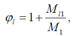 |
(a) |
where M1 and Ml1 are respectively bending moments from the action of the full load and from the action of constant and long-term loads.
The first model predicts the required value of the CFST column outer diameter Dp1 with a minimum wall thickness of a steel pipe according to the Russian assortment “GOST 10704-91. Electrically welded steel line-weld tubes. Range”. The second model has the same input parameters but, unlike the first model, predicts the required value of the outer diameter Dp2 when the pipe wall thickness is maximum. When the pipe wall thickness takes the minimum possible value, the section diameter will be the maximum, but we will have the most economical design in terms of cost. When the pipe wall thickness takes the maximum possible value according to the assortment, the pipe diameter will be minimum. Such a design will have the highest cost, but it will be distinguished by its compactness.
When designing, a balance is often needed between the cost of the structure and its dimensions. Therefore, we also developed a third model of an artificial neural network, which uses parameters 1-4, 6, the value of the outer diameter Dp in the range from Dp2 to Dp1, and the ratio l/Dp. Based on seven input parameters, the third neural network determines the required pipe wall thickness tp . A feedforward neural network with 2 hidden layers and 16 neurons on each layer was chosen as the ANN architecture. This architecture provided an optimal balance between the accuracy of the results and the cost of machine time for training. Single-layer models, as well as models with a smaller number of neurons, led to larger prediction errors. The architecture of the developed artificial neural networks is shown in Figs. (1 and 2). The activation function of the hidden layers neurons was taken as a hyperbolic tangent.
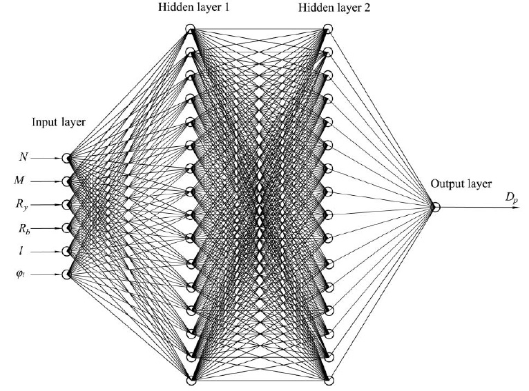
Architecture of artificial neural networks for predicting the required column diameter.
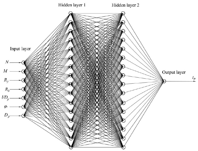
Architecture of artificial neural network for predicting the required pipe wall thickness.
| No. | Dp, mm | Min tp, mm | Max tp, mm |
|---|---|---|---|
| 1 | 102 | 1.8 | 5.5 |
| 2 | 108 | 1.8 | 5.5 |
| 3 | 114 | 1.8 | 5.5 |
| 4 | 127 | 1.8 | 5.5 |
| 5 | 133 | 1.8 | 5.5 |
| 6 | 140 | 1.8 | 5.5 |
| 7 | 152 | 1.8 | 5.5 |
| 8 | 159 | 1.8 | 8 |
| 9 | 168 | 1.8 | 8 |
| 10 | 177.8 | 1.8 | 8 |
| 11 | 180 | 4 | 5 |
| 12 | 193.7 | 2 | 8 |
| 13 | 219 | 2.5 | 22 |
| 14 | 244.5 | 3 | 22 |
| 15 | 273 | 3.5 | 22 |
| 16 | 325 | 4 | 22 |
| 17 | 355.6 | 4 | 22 |
| 18 | 377 | 4 | 22 |
| 19 | 406.4 | 4 | 22 |
| 20 | 426 | 4 | 22 |
| 21 | 478 | 5 | 12 |
| 22 | 508 | 4.5 | 24 |
| 23 | 530 | 5 | 20 |
| 24 | 630 | 7 | 24 |
| 25 | 720 | 7 | 30 |
| 26 | 820 | 7 | 30 |
| 27 | 920 | 7 | 20 |
| 28 | 1020 | 8 | 32 |
| 29 | 1120 | 8 | 20 |
| 30 | 1220 | 9 | 32 |
| 31 | 1420 | 10 | 32 |
The models were trained using synthetic data generated based on the provisions of Russian design codes for steel-reinforced concrete structures SR 266. 1325 800. 2016. Synthetic data were used because experimental data do not allow to cover the entire possible range of input parameters. Also, most of the experiments to determine the bearing capacity of CFST columns were performed on small-diameter samples. When forming training datasets, the value Dp varied from 102 to 1420 mm. The diameter values used in training the models, as well as the corresponding maximum and minimum wall thicknesses according to GOST 10704-91, are given in Table 1.
To ensure that the wall thickness is a non-decreasing function of the diameter, when forming the training dataset for model 1, the minimum thickness in row 11 was changed from 4 to 2 mm. For a similar purpose, when forming the training dataset for model 2, the maximum thickness in row 11 was changed from 5 to 8 mm, in row 21 from 12 to 22 mm, in row 23 from 20 to 24 mm, in row 27 from 20 to 30 mm, and in row 29 from 20 to 32 mm. The values that were adjusted are highlighted in bold in Table 1.
When forming training datasets for models 1 and 2, the value of concrete compressive strength Rb varied from 10 to 65 MPa with a step of 13.75 MPa (5 different values), the yield strength of steel Ry varied from 240 to 440 MPa with a step of 50 MPa (5 different values). The design column length l for each diameter value varied from 10∙Dp up to 30∙Dp in increments of 2∙Dp (11 different values). The coefficient φl varied from 1 to 2 with a step of 0.2 (6 different values).
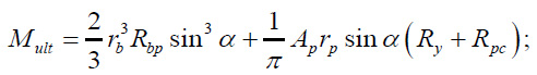
The ultimate bending moment for pure bending was determined according to SR266.1325800.2016 using the formula (Eq. 1):
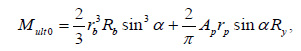 |
(1) |
where rb = (Dp-2tp) / 2 is the radius of the concrete core, rp = (Dp-tp) / 2 is the radius of the middle surface of the pipe, Ap = π Dptp and is the cross-sectional area of the steel pipe.
The angle α in Eq. 1 was determined from the solution of the equation (Eq. 2):
 |
(2) |
In addition to the ultimate bending moment, the ultimate axial force Nult0 under central compression was determined without taking into account random eccentricities and element slenderness using the formula (Eq. 3):
 |
(3) |
where Rpc = 0.75 Ry is the design strength of the pipe material under central compression, taking into account its operation in a biaxial stress state, Ab = π ⋅0.75 rb2 is the area of the concrete core, Rbp is the design strength of the concrete taking into account the effect of lateral compression, determined under central compression using the formula (Eq. 4):
 |
(4) |
Next, the step for the bending moment was selected Δ M = Mult0 / (nM - 1) , where nM is the number of calculated values of the bending moment. For each value of the bending moment M in the range from 0 to Mult0 with a step ΔM, the corresponding axial force at which the limit state occurs was calculated.
The determination of the ultimate axial force at a given bending moment was performed using a stepwise increase in the value of N from 0 to Nult0 in 1000 steps. The calculation was performed according to SR 266.1325800.2016 using the following algorithm:
1. At a given value M, the eccentricity of the axial force e0 = M / N was determined;
2. Additional random eccentricity ea was calculated as the largest of three values (Eq. 5):
 |
(5) |
3. The coefficient η, taking into account the increase in eccentricity due to the deflection of the element, was determined using the formula (Eq. 6):
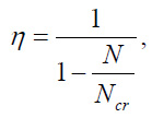 |
(6) |
where Ncr = π2 ⋅ / l2 is the conditional critical force, D is reduced cross-sectional rigidity, determined by the formula (Eq. 7):
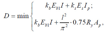 |
(7) |
where
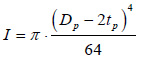 is the concrete core moment of inertia,
 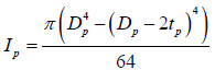 is the steel pipe moment of inertia, Es = 2.06⋅105
MPa is the steel modulus of elasticity, Eb1 is the long-term concrete modulus of elasticity, determined by the formula (Eq. 8):
is the steel pipe moment of inertia, Es = 2.06⋅105
MPa is the steel modulus of elasticity, Eb1 is the long-term concrete modulus of elasticity, determined by the formula (Eq. 8):
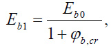 |
(8) |
where Eb0 is the concrete initial modulus of elasticity φb, cr is the creep coefficient of concrete.
The initial concrete modulus of elasticity was determined based on the paper [30] as a function of its compressive strength using the formula (Eq. 9):
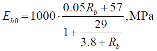 |
(9) |
Сreep coefficient φb, cr was determined using the empirical formula [31] (Eq. 10):
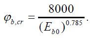 |
(10) |
Coefficients ks and kb in Eq. 7 take into account the plastic work of concrete and steel pipe. The coefficient ks is taken equal to 0.7, and the coefficient kb is calculated using the formula (Eq. 11):
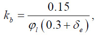 |
(11) |
where δe = (e0 + ea) / Dp is the relative eccentricity of the axial force. At δe < 0.15, the value 0.15 should be substituted into Eq. 11.
4. The calculated eccentricity of the axial force was determined (Eq. 12):
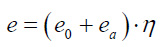 |
(12) |
5. The design strength of concrete Rbp and steel pipe Rpc under compression as part of a reinforced concrete element was determined using the formulas (Eq. 13):
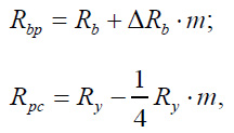 |
(13) |
where 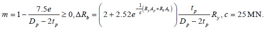
6. The angle α, which determines the size of the compressed zone of concrete in the limit state, was calculated from the solution of the nonlinear equation (Eq. 14):
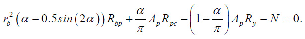 |
(14) |
7. The ultimate bending moment Mult was determined using the formula (Eq. 15):
 |
(15) |
When the product N⋅e exceeds the value Mult at the current load step, then the value N is taken as the ultimate value and written to the training dataset as an input parameter. The current value of the column Dp diameter is written to the training dataset as an output parameter. The number of calculated values of the bending moment nM when forming the training datasets for the first and second models was taken to be 41. Thus, the total volume of the training datasets for the first and second models was 31∙5∙5∙41∙11∙6 = 2097150 numerical experiments. Fragments of the generated data for models 1 and 2 are given in Tables 2 and 3.
| No. | N, kN | M, kN ∙ m | Ry , MPa | Rb , MPa | l, m | φl | Dp1, mm |
|---|---|---|---|---|---|---|---|
| 1 | 116.66 | 0.00 | 240 | 10 | 1.02 | 1 | 102 |
| 2 | 113.70 | 0.12 | 240 | 10 | 1.02 | 1 | 102 |
| 3 | 110.99 | 0.25 | 240 | 10 | 1.02 | 1 | 102 |
| 4 | 108.28 | 0.37 | 240 | 10 | 1.02 | 1 | 102 |
| 5 | 105.56 | 0.49 | 240 | 10 | 1.02 | 1 | 102 |
| 6 | 102.36 | 0.62 | 240 | 10 | 1.02 | 1 | 102 |
| 7 | 99.15 | 0.74 | 240 | 10 | 1.02 | 1 | 102 |
| 8 | 95.94 | 0.87 | 240 | 10 | 1.02 | 1 | 102 |
| 9 | 92.49 | 0.99 | 240 | 10 | 1.02 | 1 | 102 |
| 10 | 89.28 | 1.11 | 240 | 10 | 1.02 | 1 | 102 |
| … | … | … | … | … | … | … | … |
| 2097141 | 2613.60 | 9176.55 | 440 | 65 | 42.6 | 2 | 1420 |
| 2097142 | 2364.69 | 9472.57 | 440 | 65 | 42.6 | 2 | 1420 |
| 2097143 | 2115.77 | 9768.59 | 440 | 65 | 42.6 | 2 | 1420 |
| 2097144 | 1866.86 | 10064.61 | 440 | 65 | 42.6 | 2 | 1420 |
| 2097145 | 1493.49 | 10360.62 | 440 | 65 | 42.6 | 2 | 1420 |
| 2097146 | 1244.57 | 10656.64 | 440 | 65 | 42.6 | 2 | 1420 |
| 2097147 | 995.66 | 10952.66 | 440 | 65 | 42.6 | 2 | 1420 |
| 2097148 | 622.29 | 11248.68 | 440 | 65 | 42.6 | 2 | 1420 |
| 2097149 | 373.37 | 11544.70 | 440 | 65 | 42.6 | 2 | 1420 |
| 2097150 | 0.00 | 11840.71 | 440 | 65 | 42.6 | 2 | 1420 |
| No. | N, kN | M, kN ∙ m | Ry , MPa | Rb , MPa | l, m | φl | Dp2, mm |
|---|---|---|---|---|---|---|---|
| 1 | 262.64 | 0.00 | 240 | 10 | 1.02 | 1 | 102 |
| 2 | 255.79 | 0.34 | 240 | 10 | 1.02 | 1 | 102 |
| 3 | 248.37 | 0.68 | 240 | 10 | 1.02 | 1 | 102 |
| 4 | 241.52 | 1.02 | 240 | 10 | 1.02 | 1 | 102 |
| 5 | 234.66 | 1.35 | 240 | 10 | 1.02 | 1 | 102 |
| 6 | 227.24 | 1.69 | 240 | 10 | 1.02 | 1 | 102 |
| 7 | 219.82 | 2.03 | 240 | 10 | 1.02 | 1 | 102 |
| 8 | 212.97 | 2.37 | 240 | 10 | 1.02 | 1 | 102 |
| 9 | 206.12 | 2.71 | 240 | 10 | 1.02 | 1 | 102 |
| 10 | 199.27 | 3.05 | 240 | 10 | 1.02 | 1 | 102 |
| … | … | … | … | … | … | … | … |
| 2097141 | 6838.73 | 26092.78 | 440 | 65 | 42.6 | 2 | 1420 |
| 2097142 | 6154.86 | 26934.48 | 440 | 65 | 42.6 | 2 | 1420 |
| 2097143 | 5470.99 | 27776.18 | 440 | 65 | 42.6 | 2 | 1420 |
| 2097144 | 4787.11 | 28617.89 | 440 | 65 | 42.6 | 2 | 1420 |
| 2097145 | 3932.27 | 29459.59 | 440 | 65 | 42.6 | 2 | 1420 |
| 2097146 | 3248.40 | 30301.29 | 440 | 65 | 42.6 | 2 | 1420 |
| 2097147 | 2393.56 | 31142.99 | 440 | 65 | 42.6 | 2 | 1420 |
| 2097148 | 1709.68 | 31984.70 | 440 | 65 | 42.6 | 2 | 1420 |
| 2097149 | 854.84 | 32826.40 | 440 | 65 | 42.6 | 2 | 1420 |
| 2097150 | 0.00 | 33668.10 | 440 | 65 | 42.6 | 2 | 1420 |
| No. | N, kN | M, kN ∙ m | Ry , MPa | Rb , MPa |  |
φ l | Dp , mm | tp , mm |
|---|---|---|---|---|---|---|---|---|
| 1 | 116.66 | 0.00 | 240 | 10 | 10 | 1 | 102 | 1.8 |
| 2 | 105.56 | 0.49 | 240 | 10 | 10 | 1 | 102 | 1.8 |
| 3 | 92.49 | 0.99 | 240 | 10 | 10 | 1 | 102 | 1.8 |
| 4 | 79.91 | 1.48 | 240 | 10 | 10 | 1 | 102 | 1.8 |
| 5 | 67.83 | 1.98 | 240 | 10 | 10 | 1 | 102 | 1.8 |
| 6 | 55.99 | 2.47 | 240 | 10 | 10 | 1 | 102 | 1.8 |
| 7 | 44.64 | 2.97 | 240 | 10 | 10 | 1 | 102 | 1.8 |
| 8 | 33.30 | 3.46 | 240 | 10 | 10 | 1 | 102 | 1.8 |
| 9 | 22.20 | 3.96 | 240 | 10 | 10 | 1 | 102 | 1.8 |
| 10 | 11.35 | 4.45 | 240 | 10 | 10 | 1 | 102 | 1.8 |
| … | … | … | … | … | … | … | … | … |
| 2045991 | 24961.37 | 3366.81 | 440 | 65 | 30 | 2 | 1420 | 32 |
| 2045992 | 22225.88 | 6733.62 | 440 | 65 | 30 | 2 | 1420 | 32 |
| 2045993 | 19661.35 | 10100.43 | 440 | 65 | 30 | 2 | 1420 | 32 |
| 2045994 | 16925.86 | 13467.24 | 440 | 65 | 30 | 2 | 1420 | 32 |
| 2045995 | 14361.34 | 16834.05 | 440 | 65 | 30 | 2 | 1420 | 32 |
| 2045996 | 11796.81 | 20200.86 | 440 | 65 | 30 | 2 | 1420 | 32 |
| 2045997 | 9061.32 | 23567.67 | 440 | 65 | 30 | 2 | 1420 | 32 |
| 2045998 | 6154.86 | 26934.48 | 440 | 65 | 30 | 2 | 1420 | 32 |
| 2045999 | 3248.40 | 30301.29 | 440 | 65 | 30 | 2 | 1420 | 32 |
| 2046000 | 0.00 | 33668.10 | 440 | 65 | 30 | 2 | 1420 | 32 |
When forming the training dataset for the third model predicting the required wall thickness, Table 1 was used in its original form without adjustments. The range of input parameters was the same as for models 1 and 2. Since the third model contained one more parameter than models 1 and 2, the number of calculated values for the parameter φl was reduced to 5, and the number of calculated values of the bending moment was reduced to 11. The parameter l/Dp varied from 10 to 30 with a step of 4 (6 different values). The wall thickness for each diameter in the assortment varied from tp,min to tp,max with a step  (8 different values). The total volume of the training dataset for model 3 was 31∙5∙5∙11∙6∙5∙8 = 2046000 numerical experiments. A fragment of the training dataset for model 3 is given in Table 4.
Artificial neural network models were implemented in the MATLAB environment. During training, the generated datasets were randomly divided into three parts: “Train”, “Validation” and “Test” in the proportion of 70%: 15%: 15%. The mean squared error (MSE) value was adopted as a metric of training quality. Minimization of the MSE value was performed using the Levenberg-Marquardt optimization algorithm. This algorithm was chosen because it allows achieving the lowest neural network error, often with the lowest time costs [32]. The algorithm provides an acceptable compromise between the convergence rate inherent in Newton algorithms and the stability inherent in the gradient descent algorithm [33]. The number of iterations in the training process for all models was taken to be 1000 (Supplementary dataset 1-3).
3. RESULTS AND DISCUSSION
Figs. (3-5) shows the training performance graphs for models 1-3. Trained models are characterized by low mean squared error values, which are 8.96 mm2 for model 1, 7.3 mm2 for model 2 and 0.03 mm2 for model 3.
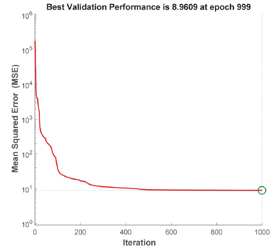
Training performance graph for model 1.
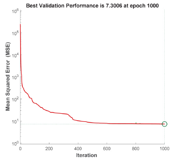
Training performance graph for model 2.
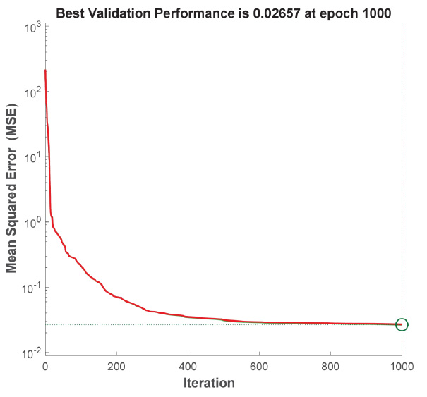
Training performance graph for model 3.
Figs. (6 and 7) show the regression plots for models 1-2. The target values T of the column diameters are plotted along the abscissa axis, and the values Y predicted by the neural network are plotted along the ordinate axis. All points on the graphs lie at a slight distance from the straight line Y = T. The correlation coefficients R between the target and predicted values differ slightly from R = 1 for the “Train”, “Validation”, and “Test” samples, as well as for the entire dataset as a whole.
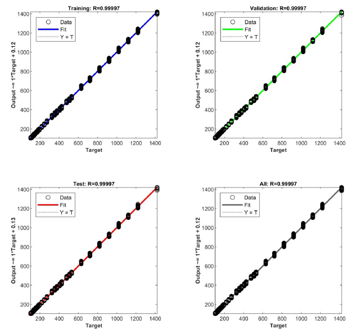
Regression plots for model 1.
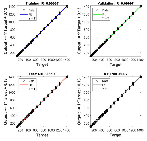
Regression plots for model 2.
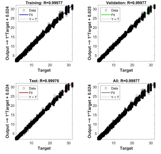
Regression plots for model 3.
| Input parameter | |||||||
|---|---|---|---|---|---|---|---|
| N | M | Ry | Rb | l | φl | ||
| Importance, % | Model 1 | 58.6 | 128.39 | 4.77 | 3.03 | 33.78 | 0.99 |
| Model 2 | 51.44 | 118.1 | 6.41 | 2.02 | 100.17 | 0.29 | |
| Input Parameter | |||||||
|---|---|---|---|---|---|---|---|
| N | M | Ry | Rb | l/Dp | φl | Dp | |
| Importance, % | 338.41 | 385.26 | 15.36 | 7.48 | 9.19 | 2.06 | 59.35 |
Fig. (8) shows the regression plots for model 3, predicting the required pipe wall thickness. In contrast to Figs. (6 and 7), the scatter of data relative to the straight line Y = T is more pronounced. This can be explained by the fact that model 3 includes one more input parameter than models 1 and 2, with approximately the same volume of the training dataset. Nevertheless, the correlation coefficients between the target and predicted wall thickness values are also close to 1. In the practical application of model 3, the engineer should round off the wall thickness value predicted by the model to the nearest one according to the assortment.
Thus, the developed artificial neural network models can act as a reliable and effective tool for determining the required cross-sectional size of eccentrically compressed CFST columns.
Machine learning methods, including artificial neural networks, also allow us to evaluate the importance of features. We chose the method of fixing values as a method for evaluating the feature's importance. The essence of this method is to calculate the relative difference between the value at the output of the neural network with a fixed value of the feature and the value at the output determined with a full set of features. As a fixed value of the feature, its average value for the entire sample is selected.
Table 5 shows the importance of the input parameters in percentage for models 1 and 2. This table shows that the values of internal forces and the design length of the element exert the greatest influence on the required value of the column diameter. The strength characteristics of steel and concrete have a lesser influence on the cross-sectional dimensions, and the influence of the coefficient φl is the most insignificant.
Table 6 shows the importance of the input parameters for model 3. Here, the least influence of the parameter φl on the pipe wall thickness is also observed. The parameters that most significantly influence the required pipe wall thickness include the values of internal forces, as well as the outer diameter of the column.
Feature importance analysis allows civil engineers to identify those parameters that can be ignored during analysis in the first approximation. In our case, this is the φl coefficient, which characterizes the share of long-term loads in the total load on the column.
CONCLUSION
Three models of artificial neural networks have been developed to predict the cross-sectional dimensions of eccentrically compressed CFST columns. The first model, based on the magnitude of internal forces, material characteristics, design length, and data on the share of long-term loads in the total load, predicts what cross-sectional diameter is required with a minimum pipe wall thickness according to the assortment of electric-welded straight-seam pipes. The second model predicts the required diameter with the maximum possible wall thickness. Having a possible range of column diameter variation, the third machine-learning model can then determine what wall thickness is required for any diameter from the obtained range. The developed models have shown high prediction efficiency based on MSE indicators and the correlation coefficient between target and predicted values. The reliability of the results is ensured by the large size of the training datasets, which included more than 2 million samples. The proposed models can be integrated into the form of utilities into existing software packages for designing building structures (CivilFEM, LIRA-SAPR, SCAD, etc.)
The importance of the features was also assessed using the variable fixation method. It was found that the required column diameter is most significantly affected by the values of internal forces and its design length. The strength characteristics of concrete and steel have a lesser effect on the cross-sectional dimensions. The required wall thickness of a steel pipe is most significantly affected by the value of the axial force and bending moment, as well as the cross-sectional diameter.
In this paper, only CFST columns with a circular cross-section were considered. However, at large eccentricities of axial forces, columns with a rectangular cross-section work more effectively on eccentric compression [34-36]. The prospect of further research may be the development of machine learning models for selecting the cross-sectional dimensions of rectangular CFST columns.
AUTHORS’ CONTRIBUTIONS
V.T. conceived and designed the study. A.C. and V.A. collected the data. S.A.Z. drafted the manuscript. All authors reviewed the results and approved the final version of the manuscript.
LIST OF ABBREVIATIONS
| ANN | = Artificial Neural Networks |
| CFST | = Concrete-filled Steel Tubular |
| AI | = Artificial Intelligence |
| ML | = Machine Learning |
| GEP | = Genetic Programming |
| GA | = Genetic Algorithm |
| SVR | = Support Vector Regression |
| SR | = Symbolic Regression |
| MSE | = Mean Squared Error |
AVAILABILITY OF DATA AND MATERIAL
The data supporting the findings of the article is available in the Yandex Disk at https://disk.yandex.ru/ d/p-5RKsDcXwTWBQ
CONFLICT OF INTEREST
The authors declare no conflict of interest. The funders had no role in the design of the study; in the collection, analyses, or interpretation of data; in the writing of the manuscript; or in the decision to publish the results.
ACKNOWLEDGEMENTS
The authors would like to acknowledge the administration of Don State Technical University, Russia for their resources and financial support.