All published articles of this journal are available on ScienceDirect.
A Genetic Algorithm with Zooming for the Determination of the Optimal Open Pit Mines Layout
Abstract
A Genetic Algorithm (GA) with nested zooming strategy is proposed for the determination of the optimal open pit mine design.
Different genetic procedures are applied to increase robustness, namely two typologies of admissible mutations for the elite sub-population subjected to zooming and mutation and reproduction for the remaining individuals. In order to further improve convergence rate, a user-defined population percentage, depending on individuals fitness, is replaced with new phenotypes, enforcing chromosomic renewal.
Several comparisons with (traditionally used) dynamic programming approaches are provided both for 2D and 3D open pit mines. Both small and large scale mines are analyzed, to benchmark the code in presence of several variables.
Results show that the procedure proposed requires a very limited computational effort, both for challenging problems with several variables and when a micro-GA (populations with few individuals) is adopted for small scale problems.
1. INTRODUCTION
The so called “open pit mining problem” [1 - 4] consists in the determination of the contour of a mine at the end of its life, which maximizes mine economic value, satisfying stability and excavation constraints. Mine stability is related to the maximum inclination of the edge of the excavated region and is strictly connected to the typology of rock considered.
One of the most interesting challenges related to this topic is the ability to solve practical problems with sufficiently large data sets and to adjust the initial solution at different periods following different scenarios based on markets evolution [5, 6]. Whilst this latter problem is extremely complex and out of the present scopes, it is worth noting that a real time adjustment requires in any case as preliminary an efficient and reliable software for the determination of the final excavation layout (at fixed input parameters).
Reliable codes are nowadays available for practitioners, usually based on dynamic programming, moving cones and integer programming strategies. In all these cases, the so called “block model” is used. A block model consists into the discretization of the open pit with small parallelepipeds, each one uniform from a geological, mechanical and economical point of view.
From a mathematical point of view, the open pit mining problem belongs to the wide class of integer programming, therefore general operational research strategies based, for instance, on branch and bound should be attempted.
Nevertheless, traditional approaches adopted by engineers (and still very diffused) are based on the so called dynamic programming (DP) technique. DP is probably the first semi-automatic method proposed in the technical literature [3]. It consists of a forward pass, in which an economic pit value Pij for each block is determined with its dependence with respect to previous column blocks. The blocks are examined level by level within each column, proceeding column by column in the section. A backward pass is also required, in which blocks dependences are evaluated step by step from the last column, giving at the end the optimal layout of the pit. Starting from the pioneering work by Lerchs and Grossman [7], who proposed a dedicated 2D dynamic programming approach also known as LG method, a number of improved dynamic programming algorithms have been proposed in the past for the analysis of 3D open-pits [8- 10].
Despite their well-known capabilities in solving medium and large scale problems, DP methods and LG in particular present some practical limitations which justify new efforts to provide alternative strategies for the resolution of the open pit mining problem. In fact, LG method performs well for 2D problems, but its generalization to the 3D case is not trivial. On the other hand, it is well known that DP requires particular care in the 3D case, as demonstrated by Shenggui and Starfield [11], who shown that a degeneration can occur in the Koenigsberg algorithm due to an over constrained formulation of the problem.
In order to avoid DP limitations, researchers focused on new strategies, essentially based on an association of DP and minimum removal cones, see Wilke and Wright [10].
A successful idea is the adaptation of 2D algorithms to the 3D case. However, if a 2D DP without minimum removal cones (Lerchs and Grossman [7]) is utilized on consecutive sections into a 3D pit, a so called “smoothing” of the pit boundaries is required. When DP is used and when the geometric constraints are specified too strictly, the pit limit will result not optimal. On the contrary if constraints are specified more loosely, the computed pit contours will require a smoothing. Different smoothing processes have been proposed in the past, as for instance the so called colour graphics approach [11], resulting promising but somewhat heuristic and not completely automatic.
Minimum removal cones strategy is the core of the algorithm known as “moving cone (MC) technique”. In the MC procedure, each ore block is considered in sequence, starting from the surface of the mine. For each ore block, the so called “minimum removal cone” is constructed, consisting in the minimum collection of the blocks of the mine (according to slope stability constraints), permitting to excavate the block under consideration. If the sum of the economic values of the blocks contained in the reverse cone is positive, the cone is considered removed. The procedure is continued until all the ore blocks in the model are examined. The ultimate pit is formed by the shape left after the removal of all positive valued cones. Despite MC simplicity, a strong limitation is clearly the aprioristic assumption of the search order for positive valued blocks, resulting in some cases into incapacity to recognize the true maximum pit value.
Against traditional approaches proposed by engineers, general mathematical concepts from optimization theory may be used to tackle the problem, which is indeed a specific integer programming (IP) problem, for which automatic branch and bound algorithms [2, 12, 13] are nowadays at disposal. Nevertheless, it is well known from optimization theory [12, 13] that in tree structures, number of nodes grows exponentially with the number of variables and may not even be finite. Therefore, to examine the whole tree may be very expensive and only partial searches inside the tree can be attempted. As a consequence, the procedure competes favourably in practice with alternative approaches if the partial search strategy is carefully chosen, deciding which node should be solved next and on which variable should a branch be made. Branch and bound can be avoided formulating the problem by means of a network flow algorithm [2], which allows the utilization of linear programming on the dual problem. It has been shown that the algorithm is closely related to LG one [7]. Thus, several questions arise in the 3D case, in particular when dependences between blocks are established. Of course, if a Koenigsberg approach is adopted, degenerations may occur, suggesting its association with minimum removal cones, thus bringing back to Wilke and Wright [10] idea.
In order to avoid all the aforementioned drawbacks and limitations, here a meta-heuristic approach based on Genetic Algorithm (GA) is proposed for predicting the optimum pit layout of both 2D and 3D mines. Particular emphasis is put on large scale examples, with the aim of testing the practical capabilities of the method, both in terms of convergence to the optimal solution and time required for the simulations.
At a first glance, the economic value of the blocks is fixed during the excavation from geological/geophysical inspections. In practice, it would be much more realistic if it could change when the excavation profile varies, but this would lead to a different, more complex optimization problem. The use of the total undiscounted economic value of the mine as objective function, calculated as the sum of economic values of the blocks to remove, is indeed a limitation, at least from the viewpoint of a mining engineer. It would be interesting to take into account the extraction schedule that aims to maximize the Net Present Value (NPV) of the mining project [14], combining within the algorithm open-pit final limits and extraction scheduling in the optimization procedure [15], thus helping in the direction of practical applications; however, such achievement is over the scopes of the present implementation, which should be regarded as a preliminary study on optimal open pit layouts by means of meta-heuristic approaches. Future developments of the model will include the implementation of extraction schedule issues.
Whilst the application of stochastic search methodologies is not new both in slope stability [16, 17] and mining engineering [18, 19], the GA proposed here is a non-standard one and allows a relatively quick convergence to the optimal solution showing excellent stability and robustness, both in case of problems with many variables and enforcing the GA to work with small populations (micro-GA).
A nested zooming strategy, consisting in the subdivision of the population at each iteration into two sub-groups, depending on individuals grade of fitness (elitist strategy), is the core of the procedure proposed. Different genetic operations are applied to the sub-groups, consisting of both two different admissible mutations for the elite sub-population and mutation and reproduction for the remaining individuals. A user-defined population percentage, depending on individual fitness, is replaced with new phenotypes at each iteration, enforcing chromosomic renewal and hence allowing a further increase of the convergence rate.
The approach is fast (very simple computations are typically required in any GA, therefore problems with many unknowns can be tackled efficiently) and generally very reliable.
However, the intrinsic GA nature (which belongs to the wide family of meta-heuristic approaches) is to provide in some limited cases suboptimal solutions. This drawback cannot be avoided, it is typical of any GA and must be checked re-running the analyses several times, to estimate how many times the algorithm provides suboptimal solutions.
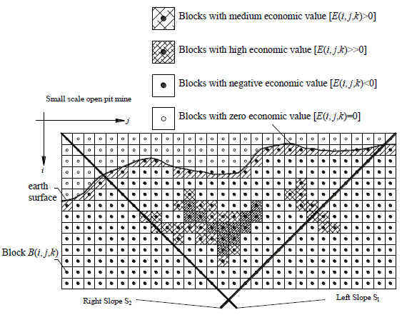
Typical 2D discretization of a mine using square blocks with slope angles constraints.
Degeneracy can occur in rare events as well, in particular enforcing limit values for GA input parameters (e.g. in micro-GAs, very high or very low values of zooming and mutation, very small initial populations, etc.). Again, it cannot be avoided in principle, but assuming reasonable values for GA input parameters degeneracy occurrence (as well as convergence to suboptimal solutions) turns out to be rather improbable.
To benchmark the model, several comparisons with previously presented results obtained with dynamic programming are provided both for 2D and 3D problems. Simulations show that reliable results can be obtained at a very limited computational effort.
2. ULTIMATE OPEN PIT MINE DESIGN: BASIC ISSUES
A rectangular block large enough to cover the area of interest is placed around the mineral deposit, Fig. (1), and further discretized into smaller blocks, generally of various sizes and shapes, but constituted by the same material with a well-defined economic value. There are various types of block models [4], nevertheless the regular 3D fixed block is the most commonly used. The pit design problem relies in finding the collection of blocks to remove which will assure the maximum profit, subjected to mine stability and mining constraints. For the sake of simplicity here cubic blocks are used with a maximum slope angle equal to 45° (i.e. 1:1 slope stability criterion). Here, it is worth noting that the assumption of a 1:1 slope criterion is not a limitation for the GA approach proposed hereafter. As a matter of fact, any slope stability rule can be used without any limitation, the effect being only a change into the cross section of the blocks, which is square in case of a 1:1 slope stability constraint and rectangular otherwise.
Let’s indicate with B(i, j, k) a block with economic value E(i, j, k) positioned on a (i, j, k) grid into a P pit. Let PA is a 3D matrix of dimensions ni × nj × nk (ni, nj and nk number of subdivisions along i, j and k) representing slope stability constraints and assuming integer values at each block B, such that:
 |
(1) |
with PA(i, j, k) = 0 if B(i, j, k) is impossible to excavate under slope constraints and 1 otherwise.
For each B(
 , j, k) block immediately under the last block excavated in position (j, k), the following mining constraints involving block B(
 , j, k) and its neighbours must be satisfied, (Fig. 2):
 |
(2) |
With reference to Fig. (2) block
 along the height of the open pit (index i) must be excavated in such a way that its neighbours are either less (i, -1) or more (i, +1) excavated by a unit.
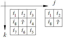
Cell (j, k) neighbours in the 3D case. Case A: case 1 < j < nj 1 < k < nk. Case B: case j = njk = nk.
Obviously, if a block is on the mine boundary column, i.e. j = 1; nj and/or j = 1; nk, ( 2 ) requirements reduce from 16 to 2nk inequalities (nk: number of neighbour columns).
Let’s indicated with Pjk the economic value of all the blocks excavated in column (j, k), i.e.:
 |
(3) |
According to equations ( 1 )-( 3 ), the ultimate open pit optimization problem can be written as:
 |
(4) |
( 4 ) is a linear integer programming problem.
3. THE 2D/3D GA PROPOSED
The reproduction of optimal open pits can be easily tackled with genetic schemes [20 - 23], avoiding in this way the utilization of DP, MC and integer programming. The advantage is represented by (a) the theoretical simplicity, (b) the robustness and efficiency in terms of time required for the optimization and (c) its applicability to large scale 2D/3D problems.
Differently from DP, the assumption of cubic blocks and 1:1 slope stability does not imply a loss of generality, because individual generation depends only on random processes based on simple admissibility inequalities which can be changed case by case, whereas selection occurs only on the base of individual fitness evaluation.
The kernel is similar to that adopted in a different context by the author in [24 - 28], where the reader is forwarded to have a detailed insight into specific technical issues. Here it is worth noting that the GA adopted relies into standard (reproduction, crossover and mutation) and non standard genetic operations [29, 30], namely zooming and elitist strategy.
Each individual is an admissible ultimate open-pit surface, i.e. a sequence of (i, j, k) blocks. Individual encoding by means of binary strings results particularly easy and the genotypes (chromosome values) are uniquely mapped onto the decision variable (phenotypic) domain. In Fig. (3) a sketch of the kernel is represented.
In a preliminary Step (0) a random admissible initial population x = {xi : i = 1,…, Nind | xi admissible} is generated. The issue related to admissibility is interesting and discussed hereafter in the paper.
In Step 1, xi individual fitness F(xi) is evaluated as the economic value of the open-pit assuming as xi the ultimate surface. In the second Step (2), which is properly known in the literature as zooming, two sub groups are formed, x̅ = {x̅i : i = 1,…, Nelit | x̅iM admissible} and y = x - x̅ = {yi : i = 1:,…, Nind-Nelit}, so that x̅ collects Nelit (user defined) individuals with high fitness.
Step 3 works on both x̅ and y. When dealing with the elite sub-population (3a), for each xi individual, a random improvement is attempted, applying two different mutation operators (1st and 2nd type). The new xiM individual resulting from mutation overwrites xi only if its fitness F(xiM) is greater than F(xi). A new sub-group x̅M = {x̅iM : i = 1,…, Nelit | x̅iM admissible} is thus obtained, with higher fitness. When dealing with the small fitness sub-population y (3b), for each yi individual, 1st type mutation is applied Nmut times, leading to an improvement of yi fitness. The new individual yiM overwrites yi based again on the better fitness criterion. Reproduction is applied only on a portion of yM (i.e. on (Nind-Nelit)/ ρ) parents with user defined parameter ρ > 1), creating new c offsprings. yM individuals excluded from reproduction are ex-novo generated with the same principles used in Step 0 and recorded into cN = {cNj : j : 1,…, (Nind-Nelit)/ ρ | cNj admissible}. At the end of the i-th iteration, a new population x = [x̅M c cN] is obtained (Step 4).
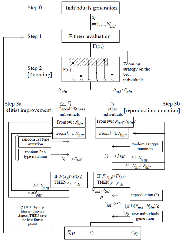
Pseudo-code of the GA proposed.
3.1. Admissible Individuals
The generation of admissible individuals requires not violating any admissibility condition. 3D and 2D implementations are conceptually identically and slight differences occur in practice, therefore here particular emphasis is given to the 2D case for the sake of clearness. Considering the 2D deposit in Fig. (4), where B(i, j) is a block in position (i, j), it can be noted that starting from the first column, in which only the block (1, 1) can be mined, different individuals may be selected at random passing successively from column
 to
to
 + 1, with
 + 1 ≤ nj and satisfying the following admissibility constraints:
 |
(5) |
where iP is the row of the deepest block mined in column
 - 1.
- 1.
 is selected with a classical roulette wheel approach, in which different probabilities are assigned at the different possible path choices, depending on the economic value of the block to remove.
In particular, the probability Pblock of each block is evaluated by means of the following formula:
 |
(6) |
Where NM is the total number of possibilities in column j, Ej is the economic value of block B(i, j) and kr is a set of constants which can be differently calibrated case by case, but which generally assume the following values
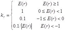 |
(7) |
In this way, a substantial improvement of the local quality (in terms of economic value) is obtained for each individual.
As a rule, for the 2D case and assuming a 1:1 slope stability constraint, only 5 different admissibility rules hold, as shown in Figs. (5, 6). Nevertheless, in the code, an automatic generation of admissible individuals is possible without the particular assumptions deduced in Fig. (4) for a 1:1 slope stability constraint. In fact, once that matrix PA is at disposal, a rectangular vector Ppos of dimensions 1xNpos is generated, representing all the admissible possibilities to select. More in detail, each element of Ppos is an admissible i index that can be assumed by the ultimate open-pit surface in correspondence of column (i , j) and Npos is the total number of admissible indices.
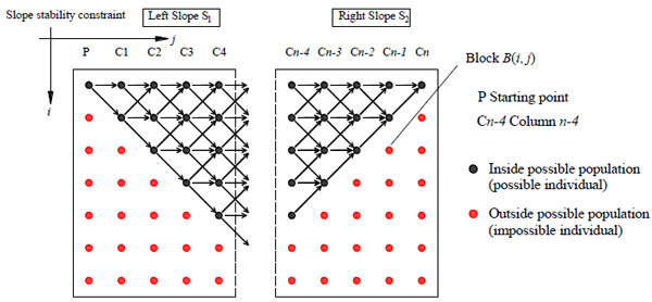
Possible tree structure of an open pit (branch and bound approach). From left to right arrows indicate admissible blocks at each column.
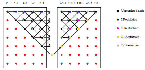
Restrictions at each block due to slope constraints, 2D case. Black points: unrestricted. Blue points: surface restriction. Purple points: right slope restriction (double possibility). Yellow points: right slope restriction (univocal choice). Red points: zone not removable.
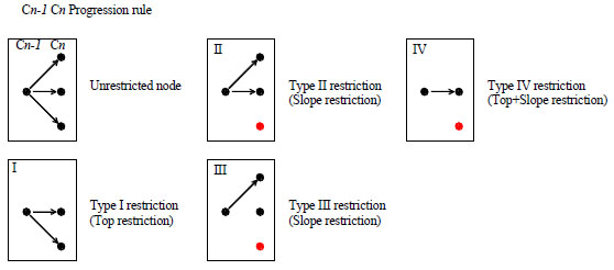
Progression rules from column Cn - 1 to column Cn, 2D case.
Matrix PA is easily obtained making used of a robust graphical 3D pre-processor implemented into MatlabTM [22]. As a rule, slope stability constraints are user defined and are pre-processed importing dxf files in which slope stability constraints are modelled with triangular/quadrangular planar surfaces, Fig. (7). Even complex geological situations can be treated with the model at hand, simply checking in the pre-processing phase for each block of the mesh if its centroid lays in the admissible region.
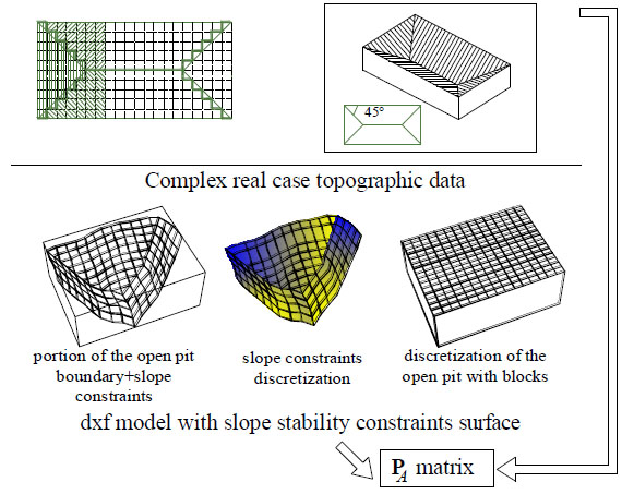
3D slope stability constraints in case of stability angle equal to 45°. GUI kit for the determination of PA matrix (data from dxf to Matlab).
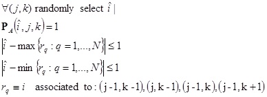
Finally, it is worth noting that, for what concerns the 3D case, the generation of admissible individuals is tacked analogously to the 2D case. In particular, individuals are generated randomly with a double loop on j and k indices and checking admissibility conditions of column (j, k) only with respect to previously filled cells (i.e. (j - 1, k - 1), (j, k - 1), (j - 1, k) and (j - 1, k + 1)), making use of the following rules (see also Fig. 8):
 |
(8) |
Obviously, equation (8) does not hold for columns j = 1 and k = 1.
The recursive application of equation (8) assures the generation of an admissible individual also in the 3D case.
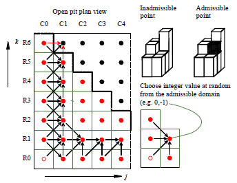
Generation of an admissible individual during the generation process in the GA, 3D case.
3.2. Reproduction, Zooming, Mutation, Crossover and Objective Function
Reproduction, zooming, crossover and mutation are relatively standard and already utilized by the author in other contexts [24-28]. For this reason here only a concise review of some technical details is provided.
Reproduction is applied only to y = {yi : i = 1 : Nind-Nelit}, mating individuals with high fitness. A stochastic sampling with replacement (roulette wheel) is utilized.
Only an offspring per pair is generated and (Nind-Nelit)/ ρ reproductions are allowed.
Zooming consists in collecting at each iteration high fitness individuals into an “elite” sub-population x̅ (with user defined dimension Nelit), where high probability mutation is applied in order to improve further fitness. Elitism preserves the original individual if mutation results into a fitness reduction, whereas zooming restricts search domain, so improving in any case convergence rate.
Zooming is a-priori set user defined through zooming percentage z%, defined as the percentage ratio between x and x̅
 |
(9) |
It is worth noting that z% can be changed according to pre-established rules, iteration by iteration. However, this is not done here, because the rule to follow for a dynamic zooming change is not either a-priori known or deduced from robust scientific bases.
Intermediate recombination (crossover) used in the paper is linear, i.e. the offspring O1 is obtained from parents P1 and P2 as follows:
 |
(10) |
Where α is an integer fixed scaling factor, which in some cases can be chosen randomly.
Considering two different individuals, here denoted as G1 (fitness F1) and G2 (fitness F2), such that Gr = {(i, j, k) | j ≤ nj ; k ≤ nk ; i admissible}, intending as admissible all those i indices satisfying slope constraints and mining stability, C12 offspring is simply generated as weighted linear combination between G1 and G2, (see Fig. 9):
 |
(11) |
Finally, C12 fitness is evaluated; when one of the parents fitness is higher than that of the offspring, parent existence is preserved (survival of the elitist).
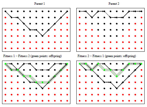
Reproduction phase (weighted reproduction) from two parents with different fitness.
1st type mutation is applied both to x̅ and y. On x̅i (associated matrix Gi(j, k) =
 ), it is repeated Nmut times randomly selecting a column (j, k) of the pit and changing in the admissible domain the value
 of matrix Gi as follows:
 |
(12) |
where
 is an integer which denotes the new admissible row of the last block to be removed for column (j, k). Obviously admissibility conditions must be checked to avoid individual inadmissibility, (Fig. 10a:)
 |
(13) |
Where rN is the number of neighbours of column (j, k), (Fig. 2).
2nd type mutation is applied only to x̅, to obtain a further fitness improvement. It works analogously to 1st type algorithm, with the only difference that two neighbouring cells (j, k)-(j, k + 1) of Gi matrix are randomly changed (Fig. 10b), according to the following rule:
 |
(14) |
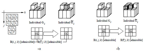
Mutation in the 3D case. (a): first type mutation. (b): second type mutation.
Obviously the new pair of integer values (ĩ1, ĩ2) has to be admissible.
In this second case, each mutation iteration consists in trying a mutation of a pair of neighbouring cells in all the possible directions, i.e. also pairs (j, k)-(j, k - 1), (j, k)-(j - 1, k), (j, k)-(j + 1, k), (j, k)-(j + 1, k + 1), (j, k)-(j - 1, k - 1), (j, k)-(j + 1, k - 1) and (j, k)-(j - 1, k + 1) are considered.
Nmut 2nd type mutations and 8 Nmut operations, i.e. all possible pair permutations, are performed. Final result of the application of both first and second type mutation is a new admissible individual (Fig. 11) x̅iM with improved fitness.
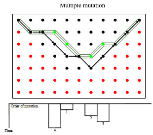
Typical result of a Nmut loop of first type mutation operations on a 2D individual.
Objective function to maximize is the total economic value of the mine. It is worth noting that, once that an admissible Gi(j, k) is selected, ( 4 ) becomes unconstrained by definition:
 |
(15) |
4. NUMERICAL SIMULATIONS, 2D EXAMPLES
In Fig. (12), a 2D block model cross-section is shown, with the corresponding solution obtained by means of the application of the LG [7] approach (numbers reported in correspondence of each cell are Pij coefficients from the recursive formula by Lerchs and Grossman [7]). The example is taken from Wright [3] to demonstrate the incapacity of the moving cone approach to reproduce the optimal open pit shape. In Fig. (13), results obtained using the present GA are shown. In Fig. (13a), the fitness value of the best individual is shown at successive generations, whereas in Fig. (13b) the optimal pit outline is traced at the last generation (numbers in Fig. (13b) indicate economic values of the blocks).
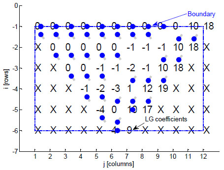
2D small scale example 1. Solution by means of the Lerchs and Grossman [7] algorithm.
The following parameters have been used: total number of individuals Nind = 6, zooming Z% equal to 50%, total number of first and second type mutations Nmut = 4, parameter ρ equal to 0.5, maximum number of generations Ngen = 50.
From a comparison between values adopted for all GA parameters and its final performance (Fig. 13), the efficiency of the algorithm is worth noting. Convergence to the optimal economic value of the pit (18 monetary units) is almost immediate, even with a micro-GA. The simulation at hand has been rerun 100 times to evaluate repeatability, finding in 2 cases sub-optimality and convergence achieved in the worst case at generation #7.
In Fig. (14), a second 2D small scale example taken from Wright [3] is reported, with the corresponding solution obtained applying the LG algorithm [7]. Also in this case, small populations have been tested (Nind = 6), with large zooming Z% equal to 40% and mutation parameter Nmut = 4. Parameter ρ has been chosen equal to 0.5 with maximum number of generations allowed Ngen equal to 50.
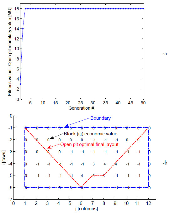
2D small scale example 1. Solution by means of the GA approach proposed. (a): best fitness value versus generation number. (b): ultimate shape of the open-pit mine.
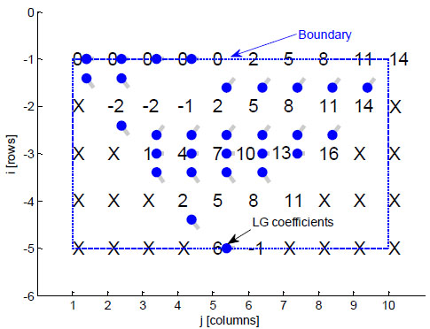
2D small scale example 2. Solution by means of the Lerchs and Grossman [7] algorithm.
Results in terms of best fitness and optimal pit outline are reported in Fig. (15). The same considerations done for the first benchmark can be repeated here. More than 200 re-runs have been performed, obtaining in the 70% of the cases an immediate convergence (i.e. after generation #1), 5/100 times subotimality and worst case convergence (14 MU) at the fourth iteration.
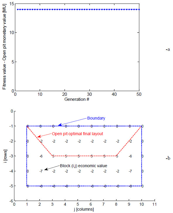
2D small scale example 2. Solution by means of the GA approach proposed. (a): best fitness value versus generation number. (b): ultimate shape of the open-pit mine.
The third example deals with a medium scale case, relying into the original Section SBHP 860001 of the Sabi Gold Project in Zimbabwe [1]. A solution is at disposal from [1], obtained both with the LG [7] procedure and the MCS/MFNN program by Frimpong and Achireko [31].
In Fig. (16), the optimal pit outline obtained applying LG [7] approach is reported, whereas in Fig. (17a, b) respectively the best individual fitness versus generation number and the GA optimal pit outline are sketched. A comparison among Fig. (17b), Fig. (16) and Frimpong et al. [1] results shows the good agreement between the final optimal profile estimated through the GA and previously presented procedures.
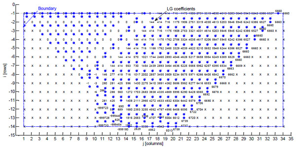
2D large scale example. Solution by means of the Lerchs and Grossman [7] algorithm.
A relatively small population has been used (Nind = 40), with medium zooming Z% (30%) and high mutation probability (Nmut = 27). ρ is equal to 0.5 with maximum number of generations allowed Ngen = 50. 200 simulations have been re-run to investigate repeatability. Convergence always occurred not over the tenth generation, with sub-optimality obtained only 4 times. Time required for the computations was usually around 8 seconds, which appears a very competitive result if compared with other approaches available.
A synopsis of economic values obtained using GA, MC and LG algorithms is reported in Table 1, for all the examples analyzed. CPU times required for the optimization on a PC equipped with 1 GB Ram and a 1.6 GHz Celeron Processor are also reported. GA simulations are repeated 100 or 200 times depending on the example, in order to have a reliable estimation of the algorithm average performance.
2D numerical simulations, comparison among CPU times needed for the optimization using the different numerical algorithms analyzed and corresponding optimized economic value found at the last iteration.
| Present Algorithm | Lerchs and Grossman [7] | Moving Cones | ||||
|---|---|---|---|---|---|---|
| CPU ime[sec] | Economic value | CPU time[sec] | Economic value | CPU time[sec] | Economic value | |
| Example 1 | 2.31/3.09 (*) | 18 | 2.44 | 18 | 1.12 | 14 (°) |
| Example 2 | 0.88/1.23 (*) | 14 | 0.81 | 14 | 0.74 | 14 |
| Example 3 / SBHP 860001 Sabi Gold Project Zimbabwe | 8/23 | 6250.8 | 21 | 6200 | 5 | 6250 |
| (*) best performance /average performance on 100
replicates (°) fails to reach the optimal solution (*) best performance /average performance on 200 replicates |
||||||
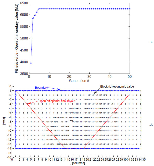
2D large scale example. Solution by means of the GA approach proposed. (a): best fitness value versus generation number. (b): ultimate shape of the open-pit mine.
4.1. Numerical Simulations, 3D Examples
A small scale 3D open pit mine of dimensions 4 × 7 × 7 (Fig. 18) already analyzed by Wright [3] by means of a number of dynamic programming approaches is discussed as first 3D example. The solution in terms of economic value is 35.5 MU [3]. In Fig. (18a and b) respectively, the best individual fitness versus generation number and the open pit optimized layout (obtained from the best individual at the last generation) are reported. The ultimate open pit layout is identical to that found by Wright [3] by means of a Koenigsberg algorithm [9] associated with MC. It is worth noting that, if a Johnson and Sharp [32] approach is used, an inadmissible optimal layout is found with economic value of the pit equal to 41.5 MU. Therefore, a-posteriori manual smoothing is needed to both reduce pit monetary value and manage admissible individuals.
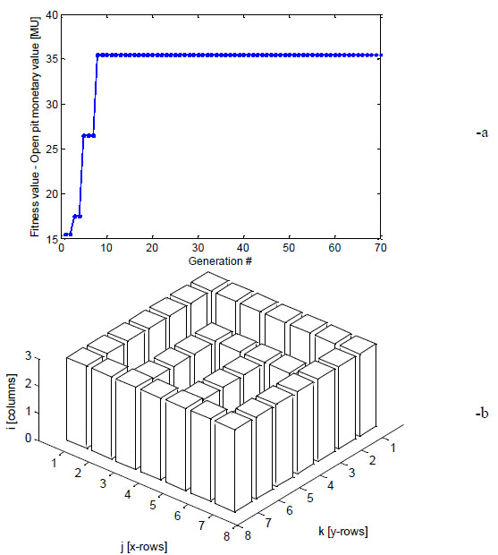
3D small scale example 1. (a): Best fitness value at progressive generations. (b): Open pit optimised layout (elitist individual at the last generation).
The GA approach proposed reaches the optimal solution automatically and efficiently (in this case, less than 5 seconds were required for the worst case simulation). CPU times required for the simulations with corresponding optimal monetary value of the pit are reported in Table 2.
A micro-GA is adopted in this case (Nind = 6), with medium zooming (Z% = 30%) and high mutation probability (Nmut = 4). ρ parameter is equal to 0.5, with maximum number of generations allowed Ngen = 70. 400 simulations have been repeated to investigate repeatability. Convergence always occurred not over the tenth generation, with subotimality found only 2 times.
The second example, Fig. (19), relies on a medium scale open pit composed by 6 × 12 × 13 blocks. Such optimization problem has been extensively studied by Wright [3], who fund an optimum monetary value of the pit equal to 111 MU, obtained using a 3D Dynamic Cone approach. 3D Level Dynamic Path and the 3D Moving Cone method slightly underestimate the maximum monetary value, providing a solution equal to 100 MU and 105 MU respectively. Sectional Dynamic Path provides a strongly underestimated optimal monetary value (89 MU).
3D numerical simulations, comparison among CPU times needed for the optimization using the different numerical algorithms analyzed and corresponding optimized economic value found at the last iteration.
| Alternative literature methods | ||||||||||
|---|---|---|---|---|---|---|---|---|---|---|
| Present Algorithm | I | II | III | IV | ||||||
| CPU time[sec] | Economic value | CPU time[sec] | Economic value | CPU time[sec] | Economic value | CPU time[sec] | Economic value | CPU time[sec] | Economic value | |
| Example 1 | 2.0/4.3 (0) | 35.5 | 3.1 (2) | 41.5 (2) | - | - | - | - | 4.1 (6) | 35.5 (6) |
| Example 2 | 12.1/14.1(0) | 111 | 11.1 (1) | 89 (1) | 6.2 (3) | 105 (3) | 9.1 (5) | 111 (5) | 13 (6) | 100 (6) |
| Example 3 | 1451 | 3250 | 731 (1) | 2991 (1) | 392(3) (4) | 3250 (3) | 991 (5) | 3200 (5) | 1212 (6) | 3200 (6) |
|
(0) best CPU
time /average CPU time on 100 replicates (1): Sectional dynamic path method (2): Johnson and Sharp without smoothing (3): 3D moving cone method (4) 3 different overlapping moving cones were used (ad hoc procedure) (5): 3-D Dynamic Cone Method (6): 3-D Level Dynamic Path Method |
||||||||||
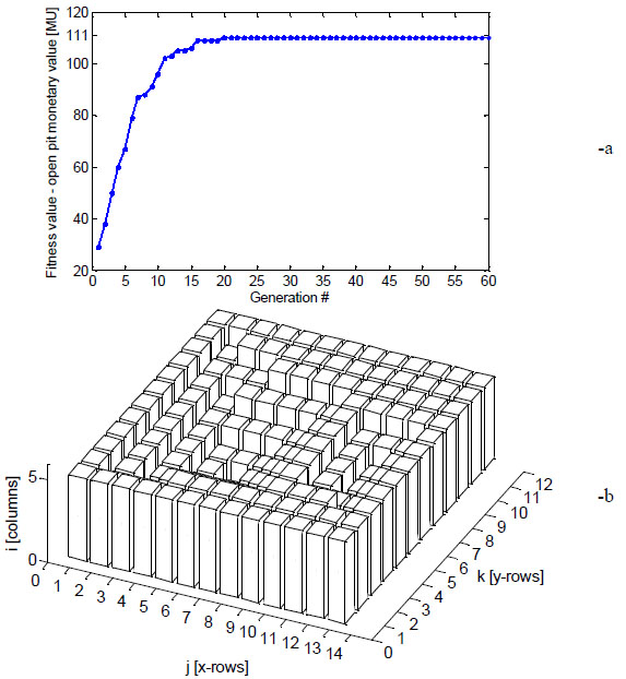
3D small scale example 2. (a): Best fitness value at progressive generations. (b): Open pit optimised layout (elitist individual at the last generation).
The performance of the GA in terms of best individual fitness at each iteration is shown in Fig. (19). For the simulations, small populations of 10 individuals, with zooming percentage equal to 30% and high mutation probability (Nmut = 4) have been used. Also in this case, ρ parameter has been set equal to 0.5 with maximum number of generations allowed Ngen = 70. Convergence to the optimal solution occurs after 20 iterations (Fig. 19a), requiring only 12 seconds, underlining again the efficiency of the procedure proposed. 100 simulations have been repeated assuming the same input parameters. Convergence was always reached before iteration #27. Sub-optimality occurred only for one simulation.
In Fig. (19b), the final open pit layout is reported and corresponds exactly to that provided by Wright [3].
The final example is a large open pit of dimensions 40 × 40 × 25, with planar external profile. The main morphological characteristic of the mine relies in a clustered distribution of blocks with relatively high economic value (varying from 10 to 20), as shown in Fig. (20). Three separated clusters with positive economic value are present, with centroids approximately located in correspondence of cells (i, 25, 35), (i, 25, 20) and (i, 12, 10) respectively. For the remaining blocks, a negative economic value equal to -0.4 is considered, exception made for the superficial blocks row (i = 1), assumed with null economic value.
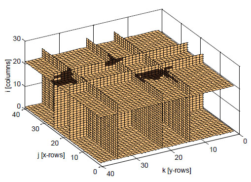
3D large scale example. Concentration of high value blocks.
From a practical point of view, each cluster could be treated separately by means of three different open pit sub-problems. Nevertheless, here all blocks have been considered in one step, with the aim of testing the efficiency of the GA for large scale 3D examples. The optimal economic value is estimated to be around 3250 MU, value calculated by means of different MCs on three separated sub-problems.
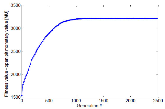
3D large scale example. Best fitness value versus generation number.
In Fig. (21) the best individual fitness at successive iterations is shown. After 1200 generations, the optimal result turns out to well approximate MC results, so demonstrating the GA efficiency for large scale problems.
The optimal outline of the open pit numerically obtained is shown in Fig. (22). Three different excavation zones can be clearly distinguished, indicating that all clusters have been mined and the optimal solution has been reached. A detailed analysis of Fig. (22) also intuitively suggests that the utilization of MC is, in this case, adequate.
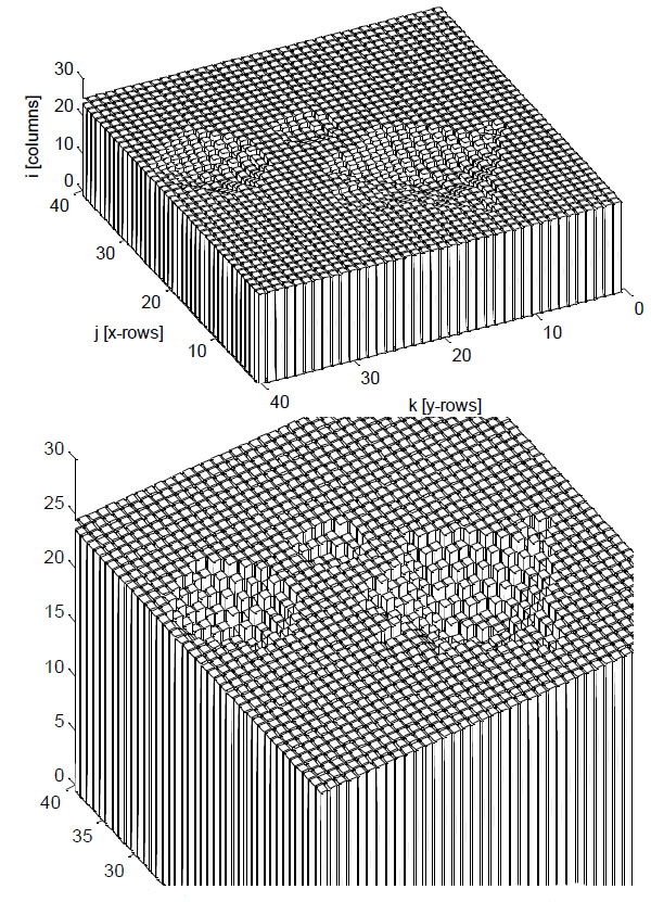
3D large scale example, open pit optimised layout.
A population with 70 individuals has been used, with zooming Z% equal to 50%, total number of first and second type mutations Nmut = 20, assuming ρ equal to 0.5 and the maximum number of generations Ngen allowed equal to 2500.
A single GA run required around 24 minutes to be performed. Convergence to the optimum economic value is acceptable, even using relatively small populations. Simulations have been rerun 50 times to test repeatability, converging always to the optimal solution (in the worst case around generation number 1350).
An additional large scale example on the same orebody of Fig. (20) has been finally performed making use of a model with 250000 blocks (Fig. 23). The mine of Fig. (23) has exactly the same characteristics of the previous orebody, except that its superficial area is around four times larger. High value blocks clusters are concentrated between columns number 1 and 40 (for both indices j and k), reproducing exactly the situation of Fig. (20). Populations with 200 individuals have been used, with zooming Z% = 50%, total number of first and second type mutations Nmut = 100, ρ equal to 0.5 and Ngen equal to 6500. The outline of the open pit numerically obtained is reported in Fig. (23). As one can note, it corresponds to the solution found for the open pit with dimensions 40 × 40 × 25. Convergence occurred after 5520 generations to a total economic value of the pit equal to 3170 MU, requiring 11 hours and 20 seconds to run. The fitness of the best individual at the last generation results in very good agreement with that obtained in the previous case.
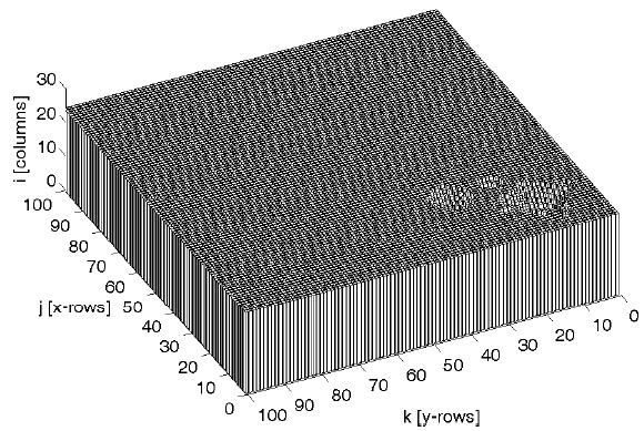
3D large scale example, simulation with 250000 blocks.
Finally, a synopsis of economic values obtained and CPU times required using GA and a number of alternative existing approaches is summarized in Table 2, for all the 3D examples discussed. Analogously to the 2D case, optimal results provided by the GA approach are obtained at CPU times always comparable with existing approaches.
CONCLUSION
A genetic algorithm for the numerical evaluation of optimal open pit mines layout has been presented. The technique exploits a specifically developed zooming strategy and survival of the fittest, based on an elitist approach. Objective function (fitness) is represented by the economic value of the pit. The reliability of the approach adopted has been assessed through meaningful comparisons with both simple cases reported in the technical literature and challenging large scale examples in two and three dimensions.
CONFLICT OF INTEREST
The author confirms that this article content has no conflict of interest.
ACKNOWLEDGEMENTS
Declared none.

