All published articles of this journal are available on ScienceDirect.
Tunnel Engineering Seepage Parameters Intelligent Back Analysis Based on FEM and Differential Evolution Algorithm
Abstract
To determine the seepage parameters of surrounding rock during excavation of tunnels, a program of groundwater seepage (SEEP) was developed. Then finite element models are established in SEEP with the consideration of seepage equations for continuous medium, and the correctness was verified by the comparison of FLAC3D. Moreover, seepage back analysis program (SBAP) was developed in C++ language by combining differential evolution algorithm (DE) and SEEP, and the measured values of water pressure and flow were used as input data, SBAP was applied to predict the horizontal and vertical hydraulic conductivities of the different stratum. The hydraulic conductivities predicted were inputted to SEEP, the computed values of water pressure and flow calculated by SEEP are in good agreement with the measured values. SBAP shows the faster convergence speed and precise feedback results. This program provides a means for engineers and researchers to determine seepage parameters in the seepage analysis of similar tunnel projects.
1. INTRODUCTION
Prediction of water inflow into a tunnel is one of the essential tasks of underground engineering [1]. Impermeable tunnel linings are almost impossible to achieve in practice [2]. Seepage is an inevitable phenomenon, which causes the potential safety threat of tunnel engineering. In order to solve the related problems, the water ingress must be somehow predicted in advance. Such predictions are burdened by a high level of uncertainty with respect to the waterhead in the ground and also the permeability of the ground [3].
The hydraulic conductivity k is the key parameter and reflects the permeability of rock mass, there are some measuring tests in laboratory such as the single-hole water pressure test and the three-section water pressure test proposed by Louis [4] in 1970, the cross-hole injection test proposed by Hsieh and Neuman [5] in 1985, and infiltration test [6] can be adopted to its identification. However, the field range is much larger than test specimen, while obtaining the parameters representing the whole seepage field demands a large number of tests, long time and cost, most direct way to identify the hydraulic conductivity at present is the field measurement methods such as pumping test and injection test unfortunately still with high cost, and these methods are not suitable for tunnel engineering because of the limitation of calculation method.
Back analysis method is an effective method to identify the field seepage parameters by the measurement information. Due to its good representativeness, wide adaptability, high reliability and fast calculation speed, back analysis has turned out to be the most efficient method to identify seepage parameters gradually.
2. RELATED STUDIES ON OPTIMIZATION ALGORITHMS
Back analysis is an optimizing problem in essence, the optimization algorithms in past were traditional and simple numerical algorithms such as golden section algorithm, simplex algorithm, newton algorithm. With the advancements of computer technology and optimization theory, many new optimization methods have been introduced into this field, including neural network algorithm [7], genetic algorithm [8], ant colony algorithm [9], Particle swarm optimization (PSO) algorithm [10]. However, there are also some disadvantages in inverse problem of seepage parameters.
All of the above optimization algorithms rely on stochastic global optimization method, a large number of random solutions are needed to evaluate the fitness of individual feature repeatedly for a better random solution. In the face of the complex structure of rock and soil, it is almost impossible to reflect the relationship between the variables and the fitness function. On the other hand, if the relationship is established through numerical calculation, the time cost will become a heavy burden, and practicality is reduced seriously [10].
Differential evolution algorithm (DE) is a new type direct global optimization algorithm proposed by R. M. Storn and K. V. Price in 1995 [11]. It has been used successfully in many fields [12-15]. This algorithm is derived from the genetic algorithm but easier to get applied without encoding and decoding operation [13]. Moreover, the correlation of multivariate is considered to a certain extent, differential evolution algorithm has a great advantage in the variable coupling problem than the particle swarm optimization [16].
In the first part and second part, the theory of finite element seepage calculation program (SEEP) and DE will be introduced, then a seepage back analysis program SBAP combined SEEP with DE is applied to tunnel engineering. The fourth part sets forth the process to use in DE algorithm to predict the seepage parameters.
The objectives of this paper are as follows:
- SEEP was combined with differential evolution algorithm to develop SBAP;
- SBAP is applied to predict horizontal and vertical hydraulic conductivity of surrounding rock of tunnel. It can be adopted to analyze groundwater seepage around a tunnel for tunnel engineering in China.
3. SEEPAGE FINITE ELEMENT PROGRAM AND DE THEORY
3.1. The Verification of SEEP
The research results indicated that the calculation results of the cracked medium model and porous medium model were not precisely the same [17]. In general, the surrounding rock is regarded as the continuous porous medium [18], the impact of cracks evenly spread over the surrounding rock. Because of the uncertainty of the joints, the associated permeability parameters are difficult to obtain by geological exploration, the surrounding rock is assumed as continuous medium which does not fully comply with the actual situation, despite all this, the continuous porous medium seepage theory is relatively mature [19], the rock mass can still be regarded as continuous medium which conforms to Darcy's law in many studies [20]. The analysis in this paper is on the basis of continuous medium, but the surrounding rock is not isotropic medium, such as slate, the hydraulic conductivity along the joint direction is larger than the vertical hydraulic conductivity. Therefore, the horizontal permeability and vertical hydraulic conductivity of model in this article can be adjusted according to actual conditions.
If water is incompressible, non-steady seepage continuity equation is as follows according to Darcy's law:
 |
(1) |
Eq. (2) can be obtained when
 .
.
 |
(2) |
Where h is the water head; x, y, z are the spatial coordinates; t is the time coordinate; kx, ky, kz are the hydraulic conductivities whose directions are parallel to the x, y, z axis respectively; Ss is the water storage rate; γ is the unit weight of water; p is the pore pressure.
The initial condition of non-steady seepage with free-surface is as follows:
 |
(3) |
Water head boundary and flow boundary are as follows:
 |
(4) |
Where, M1 is the known water head boundary; f1 is the known water head boundary value; M2 is the known flow boundary; f2 is the known flow boundary value.
The seepage finite element program-SEEP based on variation principle is developed independently, the mesh of finite element model in SEEP is generated by the preprocessing of ANSYS, then the node and element information are turned into the input file and the post-processing result displayed by visual software-Tecplot. These following assumptions are adopted according to actual engineering in this paper for simplifying [3]:
- Hydraulic conductivities are constant;
- The seepage field is in the steady flow state;
- The flow of groundwater is consistent with Darcy's law;
- The redistribution of seepage field due to the water infiltration around the tunnel.
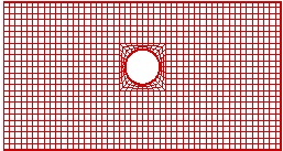
Example verification: A finite element model of the river-cross section of a tunnel is built, Fig. (1) shows the FE-mesh, consisting of 1232 quadrilateral finite elements and 1321 nodes. The boundaries of the model are permeable. The h=3m in water depth, horizontal hydraulic conductivity kx equals vertical hydraulic conductivity ky, kx=ky=0.0681m/d. The default thickness d=1m. Gradient hydraulic head pressure is applied on left and right boundaries along the direction of gravity. The same model and mesh built by FLAC3D to ensure the same coordinate of the corresponding measuring point, the calculate results can be compared intuitively.
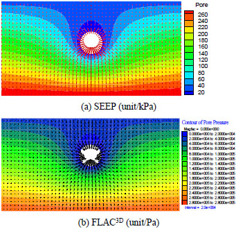
The groundwater inflow from the surrounding rock into the tunnel continuously, the distribution of pore pressure contour is typical funnel-shaped in Fig. (2) after the seepage is stable and it is consistent with the law of seepage.
The pore pressure values of each node (computed value of pore pressure) and flow values of each element can be obtained from the output file. Computed flow value of section is the sum of flow of elements around the tunnel. The pore pressure of eight randomly chosen nodes are compared with the pore pressure of nodes which have the same coordinates in FLAC3D, the maximum difference is up to 0.221%. The maximum difference of flow results of eight random elements is up to 0.840%. The difference of flow values of section is up to 1.26%. We can easily find the SEEP program can be used to obtain the accurate results of steady seepage and simulate the flow of pore water in rock mass reasonably.
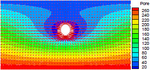
SEEP program can also solve the problem when horizontal hydraulic conductivity and vertical are unequal. Fig. (3) is the pore pressure contour in which vertical hydraulic conductivity is one-tenth of horizontal hydraulic conductivity while horizontal hydraulic conductivity is 0.0681m/d.
3.2. Differential Evolution Algorithm Theory
The development of seepage back analysis program (SBAP) is a combination of SEEP and differential evolution algorithm. Differential evolution algorithm mainly contains the generation of initial population, mutation operation, cross operation and selection operation. The major processes are as follows [11]:
3.2.1. Initial Population Generation
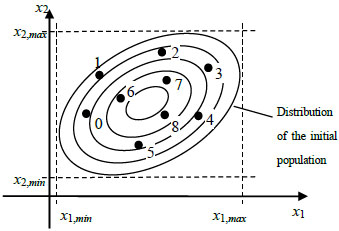
Optimization of the system means to vary the D-dimensional parameter vector, and every parameter vector is a basic individual of the evolution NP parallel vectors are generated randomly which meet the upper bound and the lower bound were shown in Fig. (4). Expressed in a formula, it can be written as follows:
 |
(5) |
Where xijU is the upper bound on j-th component of i-th vector, xijL is the lower bound. randij(0,1) denotes the random number between 0 and 1.
3.2.2. Mutation Operation
DE generates new parameter vectors by adding a weighted difference vector between arbitrary two population members to a third member and this process is known as mutation. Differential strategy is adopted in mutation operation in order to generate the variations of individuals through the individual perturbation which is reached by differential vectors among population members. Fig. (5) shows that the differential vector can be adjusted automatically according to the distribution of population members . For each objective vector of generation G+1, the j-th component of variation vector is:
 |
(6) |
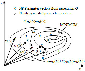
The integers r1,r2,r3 are chosen randomly from the interval (1, NP), F is a real and constant factor which controls the amplification of the differential variation, the value ranges from 0 to 1.
3.2.3. Crossover Operation
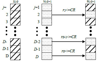
In order to keep the diversity of the perturbed parameter vectors, crossover is introduced. The objective vector xi(G) is crossed with variation vector vi(G+1) to generate a new trial vector ui(G+1):
 |
(7) |
Where rjε(0,1) is a random number corresponding to the j-th component of the vector; CRε(0,1) is crossover probability; ni is the random integral number selected from 1,2,…,D, which used to ensure one component of variation vector vi(G+1) is used by trial vector ui(G+1) at least. The whole process is shown in Fig. (6).
3.2.4. Selection Operation
To decide whether or not it should become a member of generation G+1, the trial vector ui(G+1) is compared to the target vector xi(G) using the greedy criterion, if ui(G+1) is responding to the lower objective function value, ui(G+1) selected, on the contrary, xi(G) kept.
3.2.5. Fitness Function
The objective function is used as the fitness function in DE. Setting upper bound and lower bound based on the specific physical meanings of model parameters, if there are m observation values in this field, the optimization problem of constraint is described:
 |
(8) |
Where Ai0 denotes the observed value, Ai denotes the computed value. m is the number of observed values. xi is the test parameter. xia and xib are the upper bound and lower bound of xi.
4. THE ENGINEERING APPLICATION
4.1. Hydrogeological Conditions
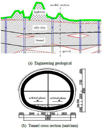
The application of SBAP in this paper is based on soil-tunnel engineering which is from Jinzhou to Pulandian in Dalian. With the length is 170 meters (DK28+345m-DK28+515m); the size of arched section is 11.20m wide and 9.05m high. The maximum thickness of covering soil on tunnel structure is 12.70m and the minimum is 4.30m. The groundwater level is 2.30m~8.00m in buried depth, the supply of water are mainly from atmospheric rainfall and river lateral feeding, runoff conditions are relatively good. The compressibility of soil is not obvious. The upper soil layer is mainly clay, the lower soil layer is gravel, and a small amount of fine sand existed in the middle. Engineering geological and the tunnel cross section are shown in Fig. (7).
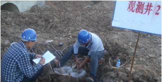
The model section is DK28+450m, the numerical analysis model is built whose surrounding soil is porous continuous medium, the width of model is 60m, and the height is 30m. The height of silty clay and gravel are corresponding to 20m and 10m respectively, the depth of groundwater surface is 6m. There are 1050 elements, 1120 nodes in the model and the quadrilateral elements are adopted for the subdivision. The boundary of the tunnel and the left, right and bottom boundaries of the model are permeable. The measured values of pore pressure of four measuring points Pi0 and flow of tunnel Fi are needed to input into SBAP. The measured values of pore pressure can be observed by piezometers near the tunnel (Fig. 8), the flow of tunnel can be calculated by the method in paper [21] which is the measured range selected near the cross section, the sum of water flows out from every drainage hole is the flow value of this section. There are two layers in this model, the upper is silty clay, with the horizontal hydraulic conductivity is Ksx and a vertical hydraulic conductivity is Ksy. The lower is gravel, with the horizontal hydraulic conductivity is Kgx and the vertical hydraulic conductivity is Kgy. In this paper, analyzing the seepage problem of surrounding soil is based on beginning after excavating and the seepage is stable, the hydraulic conductivities of grouting circle or lining are not considered. The computed value of water flow is the sum of water flows of elements around the tunnel. Table 1 shows the results of measuring points.
| Data code | measured value Pi0 /kPa | |
|---|---|---|
| Pore pressure | A | 31.39 |
| B | 44.48 | |
| C | 17.21 | |
| D | 17.36 | |
| Data code | measured value Fi0 /m3/(d/m) | |
| Flow of section | E | 1.87 |
4.2. The Solution Procedure of SBAP
Real-coded adopted in DE and the objective function f(xi), i=1, 2… n is as a fitness function in this paper. Minimizing the residual sum of squares Pi0 and Pi given by the Eq. (9) considered as the objective function, then the seepage parameters inverse problem turned into optimization problem of constraint:
 |
(9) |
The constraint condition:
 |
(10) |
Where Pi0 denotes measured pore pressure value or flow of typical section, Pi is the computed value corresponding to measured value.
DE algorithm adopted to solve the optimization problem after building the objective function and constraints, by taking the steps as follows.
Step 1: Simplified the practical engineering seepage problem to the plane seepage problem, the back analysis of the hydraulic conductivity was built based on the finite element model, which is xi=[k]T.
Step 2: There is no limit for the initial value in differential evolution algorithm, initial population generated randomly in the given range min{xil}≤xi≤min{xil}, in this paper, the range of hydraulic conductivity is set to (0,1), then the seepage finite element program SEEP was called to get Pi.
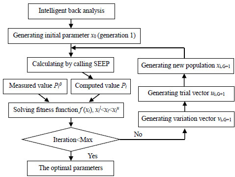
Step 3: Selecting measuring points, Pi0 and Pi of these measuring points are entered into SEEP to obtain the fitness function value f(xi). The variation vector vi(G+1) of generation G+1 is produced by mutation operation. The new trial vector ui(G+1) is generated between variation vector vi(G+1) and objective vector xi,G, selection operation is adopted between the test vector ui,G and objective vector xi,G to take xi,G+1 as the objective vector of generation G+1.
Step 4: Calling SEEP again to obtain Pi by using xi,G+1 as the inputs. The test individuals must be judged to fit the problem constraints for the availability of solutions in this process, and regression operation will be applied to the individuals which beyond the constraint.
Step 5: The crossover, mutation, selection and objective function solution operation are repeated until meeting the maximum generation number that is given, the parameter xi which minimizes the objective function is the optimal solution xi*, The solution process of SBAP is shown in Fig. (9).
 |
(11) |
4.3. Effect on Back Analysis with Different Control Parameters
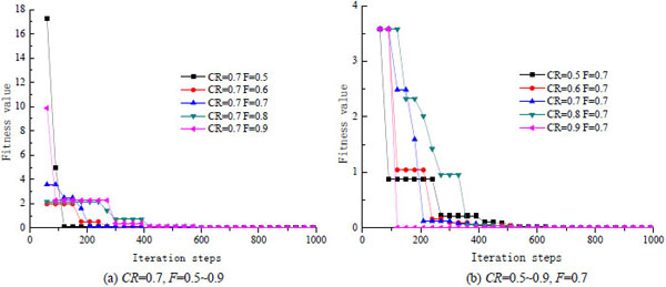
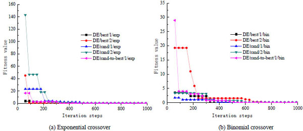
There are three main parameters in DE algorithm: population scale NP, different scaling factor F and crossover probability constant CR affect the converging property, an incorrect selection may lead to precocity and stagnation [22]. Generally NP =5D~10D (D is the number of dimensions), F=0.5~0.9, CR=0.5~0.9. This selection guarantees a high success rate of optimization, and improves the convergence speed as well. Setting four optimized parameters and thirty populations in this back analysis process. The corresponding converging curves with different F, CR and differential evolution strategies are shown in Figs. (10, 11).
All the curves in different parameters are in Fig. (10a) tend to converge while CR=0.7, F changes from 0.5 to 0.9, but the speed are different. The convergence speed is the fastest while F=0.5 which converges at about 330 step. When F=0.9, the convergence speed is the slowest which converges at about 960 step. So the appropriate search parameters selection can greatly save time and improve search speed. If F is constant, CR changes from 0.5 to 0.9, the convergence in Fig. (10b) shows the fastest speed and the highest precision while CR=0.9 and the slowest convergence speed while CR=0.5 which converges at about 810 step. CR and F should be adjusted dynamically according to the actual problems in the range and further comparison is needed to get the optimal feedback results. Price and Storn had proposed more than ten different strategies to realize mutation and crossover operation in 2003 [11]. The basic DE-strategy described in DE/X/Y/Z, where X means a string which denotes the vector to be mutated; Y is the number of difference vectors used; Z denotes the crossover scheme. The speed of convergence varied obviously with different strategies, the iterative curve in Fig. (11) shows that the convergence speed of DE/best/1/exp, DE/rand-to-best/1/exp is the fastest and more stable with exponential crossover mode, the curve converged at about 660 step. The convergence speed of DE/best/1/bin and DE/rand-to-best/1/bin is the fastest with binomial crossover mode, the curve converged at about 810 step.
The optimized parameters obtained by SBAP, ksx=0.1132m/d, ksy=0.1521m/d, kgx=0.3411m/d, kgy=0.2241m/d, are entered into SEEP to solve seepage problem, and the computed values in good agreement with the measured results in Table 2. The maximum relative error is about 2.67%.
| Differential Strategy | CR | F | Data code | Measured values Pi0 /kPa | Computed values Pi/kPa | Relative errors /% |
|---|---|---|---|---|---|---|
| DE/best/1/exp | 0.9 | 0.7 | A | 31.39 | 31.35 | 0.13 |
| B | 44.48 | 44.44 | 0.09 | |||
| C | 17.21 | 17.12 | 0.52 | |||
| D | 17.36 | 17.21 | 0.86 | |||
| Data code | Measured values Fi0 //m3/(d/m) | computed values Fi0 /m3/(d/m) | Relative errors /% | |||
| E | 1.87 | 1.82 | 2.67 |
CONCLUSION
This paper focuses on the seepage back analysis problem of tunnel excavation and surrounding rock or soil was taken as porous continuous medium; SEEP was developed based on the variation principle by C++ language. According to the boundary condition of seepage and the Darcy's law, the pore pressure of nodes and flow of element were computed in two-dimensional seepage. The correctness was verified through the comparison with FLAC3D.
Intelligent back analysis method was set up based on differential evolution algorithm, meanwhile, back analysis program of seepage parameters SBAP for short was developed independently by C++ language, which can obtain the seepage parameters successfully and predict water inflow through the pore pressure and flow value of cross section of tunnel after stability seepage. Applying SBAP to the tunnel engineering from Jinzhou to Pulandian, the iteration convergence curves shows that the feedback result is relatively better while crossover factor CR=0.7~0.9, variation factor F=0.5~0.7, differential strategy is DE/best/1/exp. The optimized parameters were entered into SEEP to get the computed valued and the maximum relative error of the computed values and measured values is about 2.67%. SBAP based on DE is feasible to solve the seepage inverse problems provide method with low cost for predicting seepage flow. This program can be used for surrounding rock seepage parameters inversion and prediction in the process of tunnel excavation, which has certain guiding significance to solve such problems.
CONFLICT OF INTEREST
The authors confirm that this article content has no conflict of interest.
ACKNOWLEDGMENTS
The authors deeply appreciate support from the National Natural Science Foundation (51678101).

