All published articles of this journal are available on ScienceDirect.

Spatial Analysis of Leakage Accidents of Oil Pipeline River Crossing Sections
Abstract
Oil pipeline leakages often bring catastrophic impacts on rivers along the pipeline, drinking water sources, and farm land irrigation etc. Based on the distinct spatial-temporal attributes in the analysis of oil spill, diffusion and consequences thereof, we present the theoretical concept and reasoning for leakage accidents spatial analysis through combining GIS and accident aftermath model. Specifically, we aim to achieve quantitative analysis and visualization of oil spill accidents through several GIS functions, which include buffer analysis, overlay analysis, spatial statistical analysis and visualized analysis. Taking a specific leakage accident of oil pipeline river-crossing section as an example, we have analyzed the polluted areas under different diffusion time and the hydrological conditions. In addition, we have evaluated populations and farm land areas affected in terms of drinking water and irrigation as well as their spatial distributions. The results demonstrate that our method can achieve quantitative analysis and visualized representations of oil spills to support policy-makers in making contingency plans.
1. INTRODUCTION
Environment is the foundation of survival and the development of mankind. Environmental pollution has become one of the most severe threats against the survival of humans. Among different types of pollution, water environment contamination directly endangers life and health of people [1]. The oil pipeline leakage is one of the main causes of water pollution. In recent years, numerous researches have been conducted across the world in water pollution accidents and Oil pipeline leakages. Wu and Alireda et al. [2, 3] carried out risk evaluations of offshore crude oil pipeline based on Bayesian Network model. Joanna evaluated the reliability and risks associated with the port oil pipeline transportation system [4]. Zhang and Zhao et al. [5-7] proposed early-warning models for river pollution contingencies based on 1D, 2D dynamics water quality model, and EFDC model, respectively. By using six-point and four-point implicit difference scheme for numerical solutions, Xu and Wu et al. [8, 9] established engineering-oriented models suitable for emergency management of sudden water pollution incidents. Through using Cartesian cut cell method, Cheng and Wu et al. [10, 11] achieved the computation of pollutant diffusion in complex river courses as well as its GIS visualization. Li and Zhang et al. [12-15] constructed water quality early-warning system after integrating GIS with water pollutant diffusion models. Anjuman and Wang et al. [16-19] undertook quantitative analyses over the impacts of oil pipeline leakages on surface and underground water. Song and Yang et al. [20, 21] statistically analyzed the causes for oil & gas pipeline failure as well as their damage on environment. Despite emerging studies on pollutant diffusion in river oil spills, few existing literature touch upon water source contamination caused by such accidents or statistical analysis and visualization of their further impacts on supply of drinking and irrigation water. To fill this void, here we present a spatial analysis approach for leakage accidents of the river crossing sections of oil pipelines.
2. MODEL FOR ACCIDENT AFTERMATH ANALYSIS
2.1. Computation Model for Leakage Amounts
During oil pipeline leakages, the maximum oil spill is comprised of spill during the responding time and maximum spill from isolated sections after valve closure, as expressed in Equation (1).
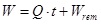 |
(1) |
Where, W denotes the maximum oil spill amounts (kg); Q represents the leaking rate within the responding time (kg/s); t denotes the respond time(s); Wrem represents the maximum spill amounts from isolated sections after valve closure (kg).
2.1.1. Leaking Rate within the Responding Time
For small hole leaking, the leaking rate within the responding time can be calculated through Bernoulli [22].
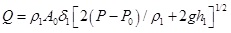 |
(2) |
Where Q denotes the liquid leaking rate (kg/s); p1 denotes the liquid density (kg/m3); δ1 is the liquid leakage coefficient, frequently from 0.6 to 0.64; p represents the pressure in the container (Pa); p 0 represents the environmental pressure (Pa), A 0 denotes the surface area of the crack(m2) by generally taking the diameter of 20% to 100%; g is the gravity acceleration rate (9.8 m/s2); h1 denotes the height of liquid level at the leakage site (m). Liquid leaking rate depends on the pressure difference between the container inside and outside.
For pipeline rupture, leakage rate within responding time equals to the pipeline oil transportation rate, as expressed in Equation (3).
 |
(3) |
Where Q denotes the liquid leaking rate (kg/s); Qtra represents the oil transportation rate within the pipeline (kg/s).
2.1.2. Maximum Oil Spill from Isolated Sections
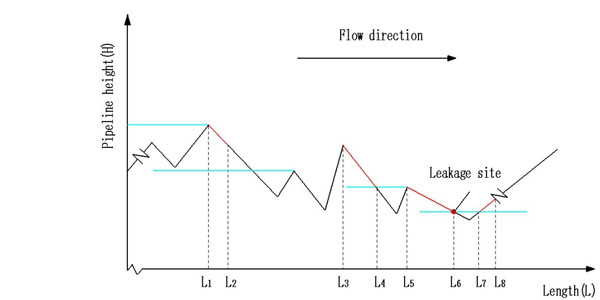
Spill of remaining oil in the pipeline after valve closure depends on the leakage site pressure, which in turn depends on the elevation of leakage site. In Fig. (1), red segments of the curve represent the pipeline sections with potential leakage. The leak detection system based on negative pressure wave could locate the leakage site, as shown in Fig. (1). Thus, the maximum oil spill from isolated sections can be calculated through Equation (4).
 |
(4) |
Where R is the pipeline radius (m); p denotes the oil density within the pipeline (kg/m3); Li (i = 1, 2, 3...) represents the pipeline length (m).
2.2. Water Pollution Prediction Model
If only considering leaked oil’s process of plug-flow transfer, dispersion and attenuation at the longitudinal direction, we can use the one-dimensional analysis model to establish a prediction model of transient emission from point-source [23]. The basic format of one-dimensional water quality model can be expressed as Equation (5).
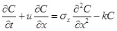 |
(5) |
Considering some factors that emission from oil spill is not stably continuous and concentration at any point is a function of time, we can derive a concentration prediction model as expressed in Equation (6).
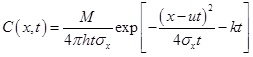 |
(6) |
where C is the pollutant concentration at the predicted site (mg/L); x is longitudinal distance between predicted site and leakage site (m); t is the predicted time (s); M denotes the total amount of oil spill (kg); h represents the average water depth of the river (m); σx is the longitudinal dispersion coefficient of the river (m2/s); u is the average longitudinal flow rate of the river (m/s); k denotes the pollutant degradation rate inside the river. As crude oil is hard to degrade, here k = 0.
Among them, river longitudinal dispersion coefficient is obtained through empirical formula based on the flat and straight river stretches. The calculation formula is as Equation (7).
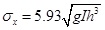 |
(7) |
Where I is the river bed gradient; g is the acceleration rate of gravity, set as 9.8m/s2.
3. PRINCIPLES OF SPATIAL ANALYSIS
Methods for leakage accident spatial analysis is mainly comprised of buffer analysis, overlay analysis, spatial statistical analysis and visualized analysis.
3.1. Buffer Analysis
Buffer analysis is the distance analysis based on the topological relationships among spatial targets (point, line, and plane). Its core idea is to specify spatial targets and define their surrounding areas, the sizes of which depend on the areas’ radii [24]. By using water quality prediction model to calculate the pollutant concentration in the water, we can derive the river pollution buffer analysis model as in Equation (8).
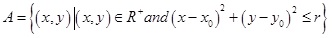 |
(8) |
Where A is the polluted river area; x 0, y 0 represent the point coordinate of leakage accident (m); r denotes the maximum diffusion distance of oil film (m); R+represents downstream river area of the leakage accident site.
3.2. Overlay Analysis
Overlay analysis seeks to generate new features or establish spatial correlations between geographical objects by overlaying two or more geographical feature layers. Once we have the polluted river areas, we can overlay it with the layer of water withdrawal sites to identify the contaminated ones. Its mathematical model is as Equation (9).
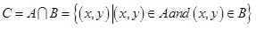 |
(9) |
Where C represents the assemblage of environmentally sensitive sites that are contaminated; A denotes the region that oil film flows through; B represents the assemblage of environmentally sensitive sites.
3.3. Spatial Statistical Analysis
Spatial Statistical Analysis is also known as Spatial Data Statistical Analysis. At its essence, the method seeks to establish the statistical relationship among data based on spatial locations as well as identify spatial dependence. Correlation, self-correlation within data related to geographical positions. Through overlay analysis, we obtain the polluted water withdrawal sites and the areas affected by accidents, then combine water withdrawal sites with topological relationship between population and farm land through spatial statistical analysis. Its mathematical model can be expressed as Equation (10).
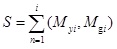 |
(10) |
Where S denotes areas affected by the accidents; Myi represents the population whose drinking water sources are polluted (person); Mgi represents the area of farm land whose irrigation water sources are polluted (Km2), i = 1, 2, 3...
3.4. Visualization Analysis
Visualization refers to the conversion of symbol or data into intuitive geometric figures that are convenient for researchers to monitor the simulation and computation processes [25]. This method primarily consists of visualized representations of map data, geographic information, spatial analysis results as well as interactive demonstration of graphs and data of analysis results.
4. EXEMPLARY CALCULATION
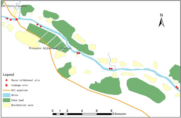
As shown in Fig. (2), the river crossing oil pipeline in our study has a diameter of D610mm and an operation pressure of 10MPa. The nearest valve chambers at upstream and downstream of river crossing section are RTU(Remote Terminal Unit)-based. Moreover, a leak detection system based on negative pressure wave is installed in the pipeline. For the purpose of spatial analysis of leakage accidents, we consider a hypothetical situation that the pipeline is ruptured due to illegal operation of a sand dredger, and regard it as small hole leaking. The river hydrological parameters are shown in Table 1.
| Season | River Flow (m3/s) | Flow Rate(m/s) | Depth(m) | Surface width(m) | River bed gradient(‰) |
|---|---|---|---|---|---|
| High-flow | 6861 | 3.77 | 10.1 | 182 | 6.3 |
| Medium-flow | 1989 | 2.12 | 6.9 | 136 | 6.3 |
| Low-flow | 43 | 0.57 | 1.2 | 63 | 6.3 |
4.1. Oil Film Diffusion Distance
4.1.1. Calculation of Leakage
The responding time between occurrence of the accident and closure of valve chambers at two ends is not more than 3 minutes. According to the leakage calculation Equation (1)-(4), p1 = 0.9kg/m2, δ1 = 0.6, p = 1 × 10⁷pa, p 0 = 1.01 × 10⁵pa, A 0 = 0.61 m2, g = 9.8m/s2, h1 = 3m, we can derive liquid leaking rate Q as 190kg/s, the total leakage within the 3 minutes responding time as 57080 kg. Meanwhile, based on the pipeline elevation parameters, we can determine the maximum leakage of isolated sections as 38860 kg. Therefore, the maximum oil spill of this accident is 95940 kg.
4.1.2. River Stretches with Excessive Pollutants at Different Times
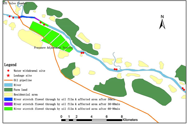
Here we assume that the pipeline’s owner launches a rapid rescue response and dispatches repair workers to the accident site within 90 min when leakage occurs. Combining water quality prediction model with buffer analysis based on GIS platform, we can determine the river stretches with excessive pollutants in medium-flow season with oil film diffusion times being 30 min, 60 min and 90 min respectively. The visualized results are shown in Fig. (3).
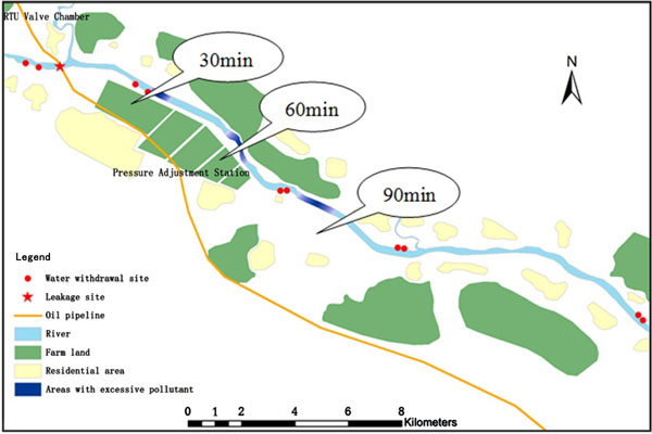
4.1.3. River Stretches with Excessive Pollutants Under Different Hydrological Conditions
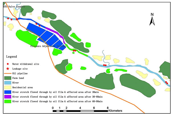
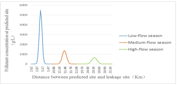
Combining water quality prediction model with buffer analysis based on GIS, we can determine the river stretches with excessive pollutants in low-flow, medium-flow or high-flow seasons with the oil film diffusion time being 90 min. The visualized results are shown in Fig. (4).
4.2. Areas with Contaminated Water Sources along River Stretches that Oil Film Flows through
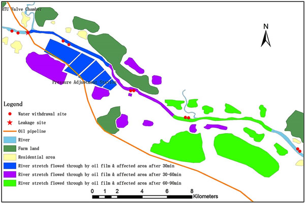
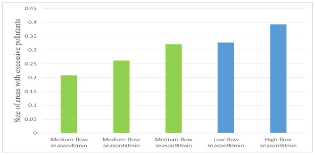
Based on excessively polluted areas, we can use buffer analysis to determine riverine regions that oil film flows through (namely contaminated regions) at different time points. In the next step, we undertake overlay analysis by superposition of affected riverine region layer and water withdrawal sites layer. On the basis of the supply-demand topological relationships between water withdrawal sites and residential areas plus farm land, we can compute the areas mostly affected by the accident. The results are visualized, as shown in Figs. (5-7). Through spatial statistical analysis, we also obtain the data of areas with affected water sources along river stretches that oil film flows through, as demonstrated in Table 2, Figs. (8-10).
| Hydrology Condition | Affected objects | Influence | 30min | 60min | 90min |
|---|---|---|---|---|---|
| Low-flow season | Resident | Drinking water | 0 | 0 | 0 |
| Farmland | Irrigation | 0 | 0 | 8.4 Km2 | |
| Medium-flow season | Resident | Drinking water | 0 | 0 | 5370 Person |
| Farmland | Irrigation | 8.4 Km2 | 8.4 Km2 | 8.4 Km2 | |
| High-flow season | Resident | Drinking water | 0 | 5370 Person | 9390 Person |
| Farmland | Irrigation | 8.4 Km2 | 8.4 Km2 | 25.1 Km2 |
4.3. Analysis and Discussion
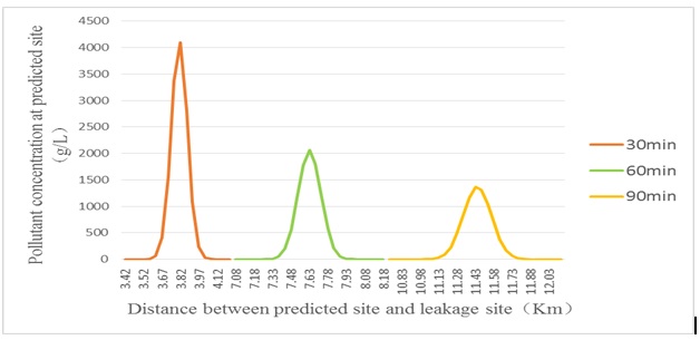
Collectively, Fig. (8) demonstrates areas with excessive water pollutant and related statistical data at different times under similar hydrological conditions. Between 30min and 90min, the oil film central diffusion distance increases from 3.82Km to 11.43Km; the oil film central concentration declines from 4095g/L to 1362g/L; Fig. (10) shows the area of regions with excessive river pollutants increases from 0.208 Km2 to 0.320 Km2. Thus, in a pipeline leakage accident oil film diffusion distance increases and maximum water pollutant concentration decreases with the passage of time. Fig. (9) shows areas with excessive water pollutant and related statistical data at the same time point but under different hydrological conditions. With the hydrological condition changing from low-flow season, to medium-flow and high-flow seasons, the oil film central diffusion distance increases from 3.07Km to 20.35Km; the oil film central concentration declines from 5487g/L to 655g/L. The size of regions with excessive river pollutants increases from 0.327 Km2 to 0.393 Km2 in Fig. (10). The results clearly show that low-flow season is characterized by the lowest oil film diffusion distance and a high maximum water pollutant concentration, indicating the difficulty of pollutant diffusion at this season. In contrast, pollutant diffusion is the easiest in high-flow season due to the highest pollutant diffusion distance and low maximum water pollutant concentration.
According to the calculation results and statistical data of areas with contaminated water sources shown in Table 2, the river stretch flowed through by oil film is the shortest in the low-flow season, in which affected area is kept at the minimum. Within 90min, none of the drinking water sources is polluted and only irrigation water for 8.4 Km2 vegetable plantation field is contaminated. The impacted area is the largest in the high-flow season, when oil film flows through the longest river stretch. Within 90min, drinking water sources for 9390 people are contaminated; irrigation water sources for 25.1 Km2 vegetable/fruit plantation fields are polluted. In the meantime, from variation in affected area during low-flow season shown in Table 2, we can infer that the size of affected area mainly depends on the number of water withdrawal sites near the oil film pollution. If no drinking/irrigation water withdrawal site exists in the stretch flowed through by oil film, the impact of pollution will mainly fall onto the river instead of resident areas and farm land.
Taken together, in a pipeline leakage accident, oil-film-polluted area largely depends on hydrological conditions and responding time of emergency repair by the pipeline owner. Moreover, in regard to areas with affected water sources along the river stretch flowed through by oil-film, their sizes mainly depend on the number of environment sensitive sites such as water withdrawal sites as well as population and farm land associated with affected water withdrawal sites.
CONCLUSION
Our spatial analysis method takes advantage of GIS to reveal the evolving process and spatial features of leakage accidents of pipeline river crossing sections. So our method can be used to enhance the scientific objectiveness and intuitiveness of pipeline/environment safety management, it could have invaluable applications in areas such as environment/ecosystems protection and water supply security.
- We have established a GIS spatial analysis method for leakage accidents of pipeline river crossing sections. The method is based on combination of the analysis model of accident aftermath with several core GIS functions, including buffer analysis, overlay analysis, spatial statistical analysis and visualized analysis. With this method, we have achieved orderly quantitative analysis and visualized representations of the complex environment, process of the beginning and development of river oil spills.
- We have elaborated the principles and procedures of the spatial analysis for leakage accidents of pipeline river crossing sections. We have also demonstrated the feasibility of the method by conducting calculation and analysis on an example. The results show that we can use this method to determine the maximum distance of oil film diffusion under different diffusion time and hydrological conditions as well as affected water withdrawal sites. By analyzing the topological relationships between water withdrawal sites and residential areas/farm land, we can ascertain the population number and farm land area impacted by the leakage accident as well as their spatial distributions.
- Compared to ocean oil spills, river oil spills are characterized by complex spatial relationship due to more complex hydrological conditions. As a result, the size of polluted region is under the influences of a diverse range of factors. Further studies can be undertaken from these perspectives to enhance the precision of accident aftermath analysis.
CONFLICT OF INTREST
The authors confirm that this article content has no conflict of interest.
ACKNOWLEDGEMENTS
This paper is sponsored by the funding project of Geographic National Condition Monitoring Engineering Research Center of Sichuan Province (GC201517), Planned Project of Science and Technology Support of Sichuan Province (2015SZ0046) and Open Fund Project of Key Laboratory of Structural Engineering of Institution of Higher Education in Sichuan Province-Methods Study of Earthquake Safety Evaluation of Oil and Gas Pipeline on Basis of Environmental Risks. Sichuan Bureau of Surveying, Mapping and Geoinformation Support Issues (J2014ZC12).