Studies on Static Frictional Contact Problems of Double Cantilever Beam Based on SBFEM

1. INTRODUCTION

The contact problem widely exists in mechanical engineering, civil engineering, hydraulic engineering, such as gear mesh, dam body joints, structural surfaces between different materials, joint and crack opening and slipping in geotechnical engineering, etc. The contact characteristics between contact bodies have great effect on the deformation, motion and stress distribution of the structure.

The prominent feature of contact problem is highly nonlinear for the contact constraints and nonsmooth for the potential energy of the contact system. Moreover, the contact boundaries are unknown in advance which make the problem more difficult to be solved. The nonlinearity of contact interfaces originates from two aspects [1]: Firstly, the area sizes and positions of contact interfaces and contact states are not only all unknown in advance, but also changed with time. Secondly, the contact conditions are nonlinear and composed by the following conditions: 1) Contact bodies cannot penetrate with each other; 2) The normal component of contact force can only to be stress; 3) The friction conditions of tangential contact. These conditions are different from the general constraint conditions, whose characteristic is unilateral inequality constraints, and has strong nonlinear property.

Contact problem belongs to free boundary problem in mathematical classification, whose analytical results are very few and difficult to be obtained for complex geometry of contact bodies and loading conditions. It is impossible to establish a perfect mathematical model to simulate the real situation and then obtain accurate analytical solution for contact problems encountered in many complex practical engineering. With rise and development of computer technology and various numerical methods, it is becoming possible to seek the numerical analysis method for the contact problem which can more accurately meet the practical problem.

As described above, the contact problem is nonlinear problem and needs to calculate in the incremental form, whose results are dependent on loading the path. Iterative method is commonly used to solve the nonlinear contact problem. Bathe and Chaudhary [2, 3] derived contact stiffness matrix for point-surface contact model by simplifying assumption, so that the stiffness matrix of equilibrium equation becomes symmetrical, and it can be conveniently solved. In order to improve computation efficiency, the contact problem can be condensed to the possible contact boundary, due to the nonlinear of contact problem mostly occurs in the possible contact area. Francavilla and Zienkiewicz [4] proposed the flexibility method whose unknown variable is contact stress based on flexibility matrix condensation. Chen [5] proposed mixed finite element method based on the contact flexibility matrix by the force method, in which the unknown variables are contact force and rigid body displacement.

Mathematical programming method is also a very effective method to solve the contact problem. In the mathematical programming method, the problem can be transformed into mathematical model that can be solved by introducing the contact constraint conditions into potential energy functional of the system. The earliest application of mathematical programming method is in the solution of the frictionless contact problem [6]. In this method, the normal non-penetration condition is introduced into the total potential energy functional of the system by Lagrange's multiplier method, and a standard quadratic programming model is formed after taking extreme value of potential energy.

For frictional contact problems, the friction force is non-conservative force and the work done by friction is embodied in the energy dissipation and does not rely on the loading path, then there is no corresponding variational principle, thus it cannot be directly equivalent to the minimization model. For 3-D frictional contact problem, the friction contact conditions are in the form of nonlinear complementary, therefore 3-D frictional contact problem should be a nonlinear complementary problem essentially. Some scholars proposed the parametric quadratic programming iteration algorithm [7], sequence linear complementary method [8] etc. in order to minimize the computational scale due to linearization as possible. Chen et al. [9, 10] proposed the nonlinear complementarity principle and smoothing algorithm for 3-D frictional contact problem. Li [11] proposed the solution of non-smooth equations for nonlinear complementary problem, which can be solved by non-smooth Newton's method. The contact problem is expressed as the B-differentiable equations by Christensen [12, 13] and solved by B-differential Newton method with guaranteed convergence property.

For contact problems, FEM and BEM are often used for the discretization of contact bodies. In this paper, the novel numerical method SBFEM developed in recently by Wolf and Song [14-17] is employed. SBFEM is a semi-analytical approach combining the advantages of finite element method (FEM) and boundary element method (BEM), and has its own characters. Only boundaries of the investigated domain are discretized resulting in a reduction of the spatial dimension by one which is similar to BEM, but the fundamental solution is not needed. These features lead to significant reduction of the computational cost. The displacement and stress fields are solved analytically in the radial direction and the accurate stress intensity factors can be calculated straightforwardly without further introducing singular elements. This method is also an excellent tool for modeling unbounded domains as the radiation condition at infinity is automatically satisfied [14]. So SBFEM is superior to solve unbounded domain and stress singularity engineering problems. This method has successfully been used in static crack propagation problems [18, 19], and in dynamic crack propagation problems [20, 21].

In this paper, SBFEM combined with the B-differential Equation is applied to deal with static frictional contact problems of double cantilever beam. The formulation for 2-D static frictional contact problem and B-differentiable equations for contact conditions are firstly presented, and the fundamental theory and details of the SBFEM can be consulted in publications [14-21]. Finally, the contact forces and deformation with different friction factors are solved and compared with those obtained by ANSYS in which FEM is employed.

2. BASIC THEORY OF SBFEM

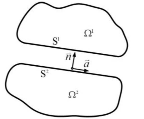
The detailed derivation and solution procedure of the SBFEM may be found in the publications [14-21] and only some key equations for the developments in this paper are summarized. As shown in Fig. (1), the domain is conveniently divided into a few super-elements whose size and shape can be arbitrary, and only the visibility from the scaling centre is considered. Only the super-element boundary is discretized Fig. (1). The SBFEM coordinates are defined as ξ and η, where dimensionless radial coordinate ξ pointing from the scaling center O to a point on the boundary, η running in the circumferential direction parallel to the boundary.

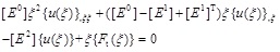
The governing equations derived using Galerkin’s weighted residual method [19] are expressed as follows:

(1)

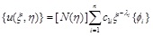
where coefficient matrices [E ⁰], [E¹], and [E²] depend on the geometry and material properties of the elements, they are independent of ξ.{F_t(ξ)}. denotes the surface tractions or loads on the side-faces. {u(ξ)} represent the nodal displacements. For homogeneous case without loads on the side-faces {F_t(ξ)} = 0, Eq.(1) is transformed into the first order ordinary differential equation. By solving the standard eigenvalue problem, the displacement field and the associated stress field inside the super-element take the form

(2)

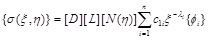(3)

where [D] is the stress-strain relation matrix; [L] is the differential operator matrix relating displacement with strain; [N](η)] is the shape function matrix.

3. BASIC DESCRIPTION OF ELASTIC STATIC FRICTIONAL CONTACT PROBLEM

3.2. Formulation of Two –Dimensional Frictional Contact Problem

For each elastic body Ω^α(α = 1,2) of the elastic frictional contact system, the boundaries S¹ and S² contain three parts: the boundary with prescribed traction S_q^α, prescribed displacement S_u^α and the possible contact boundary S_c^α. The local coordinate system are defined on the contact boundaries of body Ω², in which and are the unit normal and tangential vector.

Since the frictional force is non-conservative, the solution of contact problem is related to loading path and needs to be solved with incremental approach. At the t moment, that the equations that the elastic static frictional contact system needs to satisfy are as follows:

Equilibrium equations:

(4)

Constitutive relation:

(5)

Geometric equation:

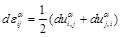(6)

Eq.(4)-Eq.(6) hold for internal point in .

In the equations above, u_i^α, σ_ij^α and ε_ij^α is displacement, stress and strain tensor respectively, du^α_i, dσ^α_ij and dε^α_ij is corresponding increment, and C_ijkl is the elastic matrix of the material.

Contact condition in the form of B-Differentiable Equations [1]:

(a) Non-penetration condition in normal direction

(7)

(b) The frictional slip condition in tangential direction

(8)

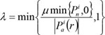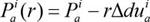Where, P_nⁱ, P_aⁱ are the total contact forces in the normal and tangential directions; r is a positive scalar; Δu_nⁱ is the normal gap; Δdu_aⁱ is the tangential incremental relative displacements; the superscript i is the i-th contact pair, NC is the number of contact pairs in the contact surface.

After the discretization of weak form of the equilibrium equation and the implementation of contact constraints, the governing equations for two-dimensional elastic static frictional contact problem can be expressed as:

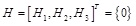(9)

where H₁ is incremental equilibrium equations expressed as Eq.(10), and H₂ ~ H₃ are B-differentiable equations of contact conditions.

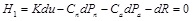(10)

In Eq.(10), dR is the incremental external force, dP_n and dP_a are the incremental contact forces, [C_n] and [C_a] are matrixes which transform the vectors of local contact forces into the global ones.

Eq.(9) can be solved by B-differentiable Newton method. In order to improve the efficiency of computation, the equilibrium equation Eq.(10) can be condensed into the Dofs of the contact points firstly, then the equations (9) and (10) are solved by B-differentiable equation method to get the contact force, finally the displacement is obtained by solving Eq.(10) with the known contact forces. The detailed solution procedures of B-differentiable equation method can be found in publications [13, 22].

4. NUMERICAL EXAMPLE

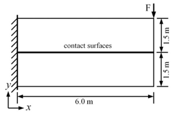
As shown in Fig. (2), the contact between two cantilever beams with the same size is analyzed. The size of each beam is 6.0m × 1.5m; the beams are fixed at left side; a concentrated load F(F = 100KN) is applied on the top right of the upper beam along the vertical direction. The initial gap between the two beams is zero and their interfaces are the potential contact areas. The material properties of two beams are the same, whose parameters are as follows: Young's modulus E = 10GPa; Poisson ratio υ = 0.3; friction coefficient µ is taken as 0.0, 0.2 and 0.5 respectively. The plane stress state is assumed, and the gravity effect of the beams is ignored. In order to verify the validity of the proposed solution procedure in the framework of SBFEM, the results are compared with those obtained by ANSYS program.

4.1. Solution of Static Contact Problem by SBFEM

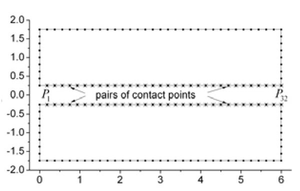
As shown in Fig. (3), for each beam only the boundaries are discretized by the three-node quadratic elements (their nodes are marked as those tiny black dots “.”, and each super-element has eighty nodes). The scaling centre is chosen at the centroid of the beam. Both beams are disretized with same mesh size and can be analyzed using the node-to-node model in which the discretized contact surfaces are mesh-matching. Two nodes with the same coordinates on the different beams are defined as a pair of contact points (marked as ‘*’) and the total number of which is 32 (P₁, P₂,...,).

4.2. Solution of Static Contact Problem by ANSYS

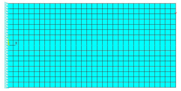
As shown in Fig. (4), the double cantilever beams are discretized with PLANE82 elements (eight-node plane element), whose total number is 1698, the surface-to-surface contact is employed. The left ends of the beams are fully constrained. The mesh size in the ANSYS is half of that in the model solved by SBFEM. The output results of 32 contact pairs are compared.

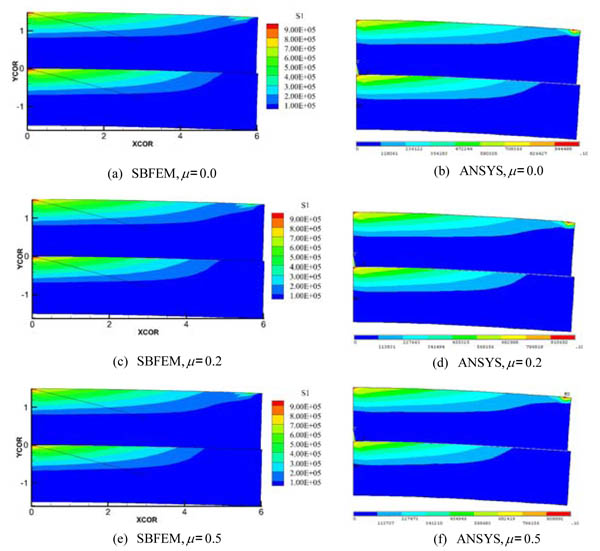
The deformation figures (magnified 100 times) with the contour of principal tensile stress σ₁ resulted from SBFEM and ANSYS for different frictional coefficients are shown in Fig. (5). It can be seen from the figures that the peak value and distribution of the principal tensile stress σ₁ are in good agreement. Besides, the upper parts of the upper and lower cantilever beams sustain tensile stress, and the peak value occurs on the left constraint of each beam. No penetration appears which agrees with the actual situation, due to the contact between the two beams is considered. As shown in Figs. (5a, 5b and 5c), by comparing the distribution of principal tensile stress σ₁ of double cantilever beams with different friction coefficients, it can be found that, for different friction coefficients, the stress distributions solved by SBFEM is consistent with those by ANSYS.

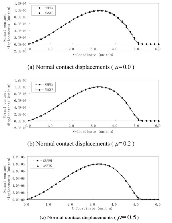
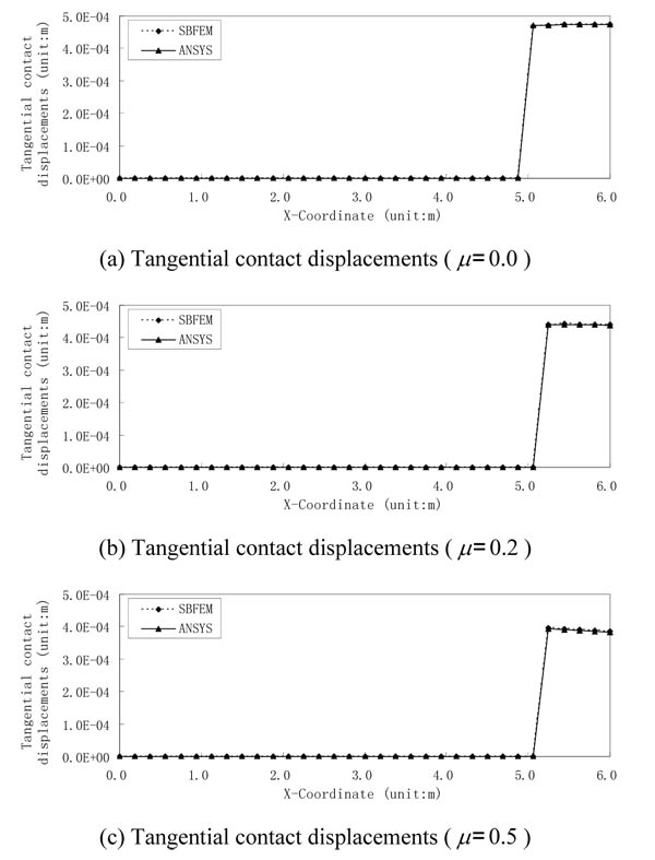
Figs. (6 and 7) show the normal and tangential displacements of contact points respectively for double cantilever beams with different friction coefficients solved by SBFEM and ANSYS. As shown in Fig. (6), normal contact displacements of each contact pair obtained by both methods are nearly identical, whose result errors are all within 5.0% except for the two pairs of contact points (P₂₆ and P₂₇) at the right side. It can also be drawn from the comparison of normal contact displacement of contact pairs with different friction coefficients (as shown in Figs. 6a-6c) that normal displacements of contact pairs are almost the same for different friction coefficients. As shown in Fig.(7), tangential displacement curves of contact pairs by both methods nearly coincide, whose result errors are all less than 0.8%. Tangential displacements gradually reduce with the increase of friction coefficient as shown in Figs. (7a-7c).

It can be seen from the normal contact displacement curves in Fig. (6) and the tangential ones in Fig. (7) that when friction coefficient µ = 0.0, six pairs of contact points (P₂₇-P₃₂) on the right side are in the contact status, while the remaining pairs of contact points are in the separation status. But when µ is 0.2 or 0.5, only five pairs of contact points on the right side (P₂₈-P₃₂) are in the contact status. In ANSYS, the distributed contact pressure, not the nodal contact force is obtained. When friction coefficient µ = 0.0, the total normal contact force by SBFEM is 53.64KN , and that is 54.52KN by ANSYS. For µ = 0.2, the total normal contact force based on SBFEM is 53.64KN, which is 53.88KN, by ANSYS, and the total tangential contact force by SBFEM is 10.73KN, and that is 10.78kN based on ANSYS. For µ = 0.5, the total normal contact force based on SBFEM is 53.64KN, and that is 54.16kN by ANSYS, and total tangential contact force based on SBFEM is 26.82KN, and that is 27.08KN by ANSYS. From the above analysis, with the increase of friction coefficient µ, tangential contact displacement reduces gradually when tangential contact force increases, and the different friction coefficients have few effect on the stress distribution, normal contact force and contact displacement.

CONCLUSION

This paper presents the formulation and solution procedure by combing SBFEM and B-differentiable equations for solving two-dimensional frictional contact problem. As an example, the contact problem of double cantilever beam is given to verify the accuracy and effectiveness of proposed method by comparison with ANSYS software. In the framework of SBFEM, only the boundaries of contact bodies are needed to be discretized with one-dimensional three-node linear elements for 2D case and the total number of nodes is far less than that in ANSYS. For different frictional coefficients, the results obtained from both methods are in good agreement. It can be drawn from the analysis that with the increase of friction coefficient, tangential contact displacement reduces gradually, while tangential contact force increases little by little, but normal contact force and contact displacement are almost constant.

It also can be found from the previous analysis that if the contact algorithm is introduced to the fracture analysis of structure, the contact between the crack surfaces will be considered reasonably.

REFERENCES