All published articles of this journal are available on ScienceDirect.
Compressive Strength and Slump Prediction of Two Blended Agro Waste Materials Concretes
Abstract
Background:
Agro industrial wastes such as Bamboo Leaf Ash (BLA) and Bagasse Ash (BA) need to be employed so as to replace cement in order to produce cheaper concrete, which, in turn, save the environment.
Objective:
This research focuses on the compressive strength and slump based on Artificial Neural Network (ANN) and Multiple Linear Regression (MLR) models for forecasting of compressive strength and slump value for concrete by blending BLA and BA as partial supplementary cement materials accordingly.
Methods:
Three-layer perceptron was constructed through R (nnet package). A sum total of eleven artificial neural networks were formulated using 214 data sets attained from 27 laboratory concrete mixtures performed.
Results:
The neural network model forecasted the compressive strength for training, testing and validation with predicted errors of 0.802 MPa and 1.380 MPa. The model over forecasted the compressive strength averagely by 0.644 MPa and 1.905 MPa. The forecasted compressive strength changed averagely by 2.328% and 3.946%. The average difference between the predicted and experimental values was 0.588 MPa and 1.050 MPa. The coefficients of determination were 0.961 and 0.905. The MLR model predicted the slump with predictive error values of 6.634 mm and 8.374 mm. The predicted slump deviated on average by 3.633% and 8.034%. The residual error was 3.075 on 12 degrees of freedom. The multiple R2 and adjusted R2 were 0.9336 and 0.9115. The P-value was found to be 5.639e-07.
Conclusion:
The results show that ANN and MLR are potent tools for forecasting the compressive strength and slump of concrete blending bamboo leaf ash and baggage ash. Hence, this contributes towards forecasting of the compressive strength and slump of BLA and BA blended concrete. They extends 28 days compressive strength usually found in the literature to 56 and 90 days compressive strength and there was a remarkable improvement as curing age increases. The slump of combined effect of blending BLA and BA at different percentage replacements was tested. In this study, we used BLA blended with BA to produce concrete which is an innovation.
1. INTRODUCTION
Concrete is a combination of aggregates and cement which could be framed to any magnitude and forms of the expected design [1]. The world’s yearly manufacturing of concrete is evaluated to be greater than ten billion tons [2, 3]. Cement manufacturing costs a lot of resources and energy. One ton of cement manufacturing depletes roughly about 1.7 tons of raw materials, 4 Giga Joules (GJ) of energy, and discharges roughly 0.73 – 0.99 tons of carbon dioxide into the atmosphere [2, 4-6]. As a result, the concrete sector is now finding means to exploit alternative elements for concrete production in order to attain sustainable growth and to reduce the harsh environmental effect [7].
Agro-industrial wastes have been employed to replace cement so as to produce affordable concrete. These, in turn, stimulates solid waste management and conservation of natural resources [8-15]. Other waste materials such as sewage sludge ash [16], nano-silica particles [17], blast furnace slag and nano silica hydrosols [18], calcined sewage sludge ash [19], nano silica and sewage sludge ash [20] have been used for replacing cement at different percentage replacements for producing concrete. Bamboo leaf ash (BLA) and baggage ash (BA) are part of the agro-industrial wastes that are utilised as promising cement replacement materials.
Traditional concrete is a mixture of water, cement, fine aggregates, and coarse aggregates [7]. The features of the concrete are affected by various factors like the type of cement, water-cement ratio, water content, quantity and quality of aggregates [21]. The conventional method employed in modelling the impacts of these factors on fresh and mechanical features of concrete begins with an assumption of an analytical equation [22]. Meanwhile, the method does not capture the real scenario when some of the concrete components are not the traditional elements and when the assumptions are wrong.
Slump and compressive strength are important fresh and mechanical features of concrete and play a vital role in the design of concrete entities [23]. Workability is the characteristic of concrete which ascertains the efforts needed for compaction, finishing, and insertion with the lowest loss of uniformity. The final compressive strength of concrete is mostly achieved after curing age of 28 days which serves as a point of reference to define the strength at the subsequent age [24, 25]. Methods like mechanical modelling, analytical modelling, artificial intelligence, multiple linear regression, and other statistical methods [7, 25] have been used lately for forecasting the slump and strength of concrete. An artificial intelligence technique which has flourished well and grown swiftly in engineering practices is Artificial Neural Network (ANN) [26, 27]. The artificial neural network has been used in lots of civil engineering practices such as groundwater monitoring, concrete strength forecasting, material behaviour modelling, discovery of structural damage, concrete mix apportioning, and structural system recognition [28, 26, 29-31].
Numerous research works [7, 21, 29, 30-34] have employed artificial neural network for forecasting the strengths of various kinds of concrete. Duan et al. [7] developed an artificial neural network model using a single hidden layer. The artificial neural network model forecasted the recycled aggregate concrete strength accurately. Chopra et al. [21] also used sigmoid activation function and Levenberg-Marquardt training function for predicting compressive strength based on ANN modelling. They found that the sigmoid activation function and Levenberg – Marquardt were the best forecasting tools. ANN predictive model was also constructed by Hossein et al. [28] for forecasting the compressive strength of the recycled aggregate concrete. The outcome of their studies revealed that 0.0044MPa at epoch 5 was the best performing validation. A multi-layer feed-forward artificial neural network architecture known as 5-10-1 was developed by Kalra et al. [35] for the purpose of forecasting the compressive strength of concrete. Based on their research, the suitable validation was noted at epoch 40 and 10.99 MPa as its mean squared error value. Jamaladin et al. [36] forecasted the compressive strength of high-performance concrete through ANN. They studied thirty ANN architectures and found that 8-10-6-1 was the best architecture for their model. Their model was capable of simulating experimental results correctly. Getahun et al. [37] also employed ANN predictive modelling for prediction of compressive strength and tensile strength using rice husk ash and reclaimed asphalt aggregate concrete.They used 15-15-2 architecture which is multi-layer feed-forward. Their actual and predicted results were very close. Heidari et al. [38] used ANN model in order to predict strength of concrete. It was discovered that the real values and the predicted values produced by neural network were closer and absolutely correct. ANN model was also constructed by Bharathi et al. [39] towards the forecasting of hardened and fresh components of self-compacting concrete by partial replacement of cement with fly ash.
Multiple Linear Regression (MLR) on the other hand is a statistical method which utilises several independent variables in order to forecast the outcome of a dependent variable. The basic work of MLR is to model the relationships that exists between independent variables and dependent variables. It has been used in civil engineering for slump prediction and strength prediction as well [40].
Charhate et al. [40] utilised MLR for the purpose of predicting the slump of concrete grade of M20, M25, M30,M35, M40, M45,M50,M60, and M70. The predicted slump value obtained for each grade of concrete was closer to the actual slump value. Yeh [41] used MLP for predicting the slump flow of high-performance concrete, the outcome of the research indicated that the differences between the actual slump and forecasted slump were minimal.
The key factor for ANN’s wide applicability and acceptance is its tendency and efficacy in resolving complicated and complex engineering setbacks [26]. Basically, the feed-forward network (multi – layer perception) has been frequently utilised in ANN architecture [42]. Feed-forward network consists of an array of extensively lateral neurons that are computational. The nodes are linked to each other by connected weights and collect the input signals based on the neurons connected together with it. Succeeding layers of the nodes obtain input from preceding arrays. That is, the output for the nodes of every array provides inputs to the nodes of the next layer. The artificial neural network processing components are analogous as compared with neurons of human brain which consist of computational segments grouped in layers [22]. Furthermore, ANN has the ability to unveil amazing potentials in the modelling of human brains [43].
There is a need to train and design the ANN accurately with data with respect to the challenge so as to obtain the required purpose. The log - sigmoid, purelin, and tan-sigmoid are the most famous activation functions [44]. Besides the output and input neurons, activation function is a key which alters the performance of an ANN [45]. Backpropagation algorithm has been largely employed for feed-forward network training [37].
The key data was obtained via laboratory experimental work for developing a compressive strength forecasting model through ANN and MLP. The combination of BLA and BA to produce concrete is a new initiative, as no study has been performed so far in this aspect. The features and constituents of concrete blending BLA and BA are clearly not the same as normal concrete, this, in turn, make it difficult to forecast compressive strength through statistical and analytical modelling techniques . The statistical model approach adopts a parametrization and premeditated pattern. Also, the analytical method is normally restrained due to some complications; it is either pointless or unduly rigorous to be formulated as a result of its illogical postulations. Conversely, ANN model has the ability to represent non – linear compounded relations between variables through examining vital features inherent in the data [37]. Furthermore, ANN can produce undesirable outcomes to impediments such as errors in the input variables which render it deficient. Hence, it has the ability to generalize and learn from occurrences and records [39]. MLP has the ability to represent linear compounded relations which exist among the variables correctly [36].
The contributions made in this paper are: (1) To affirm the efficiency of ANN and MLR models in forecasting the compressive strength and slump of BLA and BA blended concrete (2) Previous researchers worked on 28 days compressive strength. However, in this study, 56 and 90 days compressive strength was tested using ANN, there was a remarkable improvement as curing age increases. Also, the slump of the combined effect of blending BLA and BA at different percentage replacement was tested using MLR (3) Previous researchers used different pozzolans and admixtures to produce concrete. However, in our study, we used BLA and BA to produce concrete.
2.1. Elements Used
Elements employed in this studies consist of a superplasticizer, Baggage Ash (BA), Coarse Aggregate (CA), Bamboo Leaf Ash (BLA), water, Fine Aggregate (FA), and Ordinary Portland Cement (OPC). All the materials utilised were obtained from different counties in Kenya. Coarse aggregate and fine aggregate were acquired from Mlolongo and Masinga sited in Machakos county, Kenya. Sugar cane ash was fetched from sugar manufacturing industry situated in the Kakamega province of Kenya.The leaves of the bamboo were collected in a forest (MAU) situated in Kenya. The cement, as well as superplasticizer, was obtained from the central part of Kenya. Potable water from the tap was utilised.
2.2. Procedures
Table 1 shows the procedures utilised for this research work; all the methods shall be discussed in the next section.
| Constituent Elements Tests | |
|---|---|
| Conducted Test | Standard Employed |
| Sieve analysis (BLA, BA) | ASTM D7928-7 |
| Sieve analysis (Aggregates) | ASTM C33 |
| BA, BLA and cement SG | ASTM 188 |
| Fineness modulus | ASTM C136 |
| Aggregate water absorption | BS EN 1097 |
| Voids in aggregate | ASTM C29 |
| Aggregate density | ASTM C29 |
2.2.1. Test Methods for Material Classification
The grading technique for aggregates was conducted based on ASTM C 33 [46] concept by utilising sieves in agreement to BS ISO 3310-2 (2013) [47]. Aggregates’ selection was accomplished based on BS EN 932-1 (1997) [48] batching conditions. The leaves of the bamboo were dried in the sun to eliminate the liquid content present in it. Afterward, they were then subdued to burning in order to get rid of organic materials that might be present in them. Hence, calcination operation took place through muffle furnace at 650°C for 2 hours as detention time. After cooling, it was sieved through sieve size of 0.15 mm. The baggage ash was fetched from the sugar industry and was also sieved with 0.15 mm sieve size.
2.2.2. Mix Operation and Design Mix
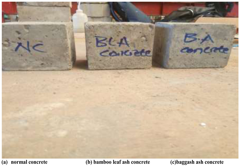
A total of 25 mixes were prepared. The details of the mix distributions are stated in Table 2. The cement was partly substituted using 5%, 10%, 15%, and 20% of BLA and BA through weight of the total cement. BLA was kept constant ranging from 5%, 10%, 15%, to 20%. BA varied from 5% - 20% and was blended with the BLA at each level of replacement. The mixtures were prepared using 195 kg/m3 water and a constant water binder ratio (w/b) of 0.5. Furthermore, 0.8% by cementitious material weight superplasticizer was employed for the mixes. Manual mixing was carried out as stipulated in BS EN 1881-125 (2013) [49] and was taken care of by a tool to shield against the dispersion of liquid and cementitious materials at the mixing stage. Chemical analysis for BA, cement, and BLA was conducted through x-ray diffraction (XRD) equipment in line with BS EN 196-2 (2013) [50]. The cement, baggage ash, and bamboo leaf ash were obtained based on ASTM C188 (2016) [51]. The concrete design mix for grade 25 was carried out with reference to BS EN 206 (2014) [52] as well as BS 8500 -2 (2012) [53].
|
Structure of the mix [BLA/BA] (%) |
BLA (kg/m3) | BA (kg/m3) | OPC (kg/m3) | F.A (kg/m3) | C.A (kg/m3) | Water (kg/m3) | Superplasticizer (kg/m3) |
|---|---|---|---|---|---|---|---|
| Concrete without admixtures | 0 | 0 | 390 | 662 | 993 | 195 | 1.5 |
| [5-20]% BLA | [19.5-78] | 0 | [312-371] | 662 | 993 | 195 | [1.482-1.248] |
| [5-20]% BA | 0 | [19.5-78] | [312-371] | 662 | 993 | 195 | [1.482-1.248] |
| 5%BLA + [5-20]%BA | 19.5 | 19.5 | 371 | 662 | 993 | 195 | 1.482 |
| 10%BLA + [5-20]%BA | 39 | 39 | 351 | 662 | 993 | 195 | 1.404 |
| 15%BLA + [5-20]%BA | 58.5 | 58.5 | 331.5 | 662 | 993 | 195 | 1.326 |
| 20%BLA + [5-20]%BA | 78 | 78 | 312 | 662 | 993 | 195 | 1.248 |
3. RESULTS AND DISCUSSION
3.1. Material Characterization
Bagasse ash, bamboo leaf ash, fine aggregate, and coarse aggregate elements were categorized with reference to grading. Also, BA, cement, BLA, and aggregates were categorized with reference to specific gravity. Aggregates werecategorized based on density (bulk), void content, water absorption as well as fineness modulus.
Table 3 displays the specific gravity of cementitious materials, fine aggregates, coarse aggregates, water absorption, bulk density, fineness modulus, silt content etc.
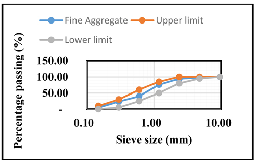
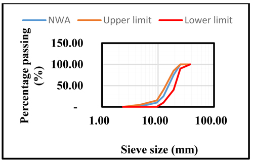
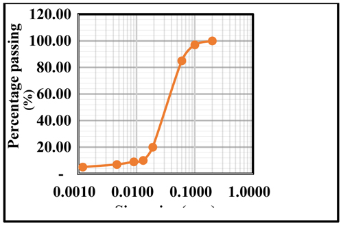
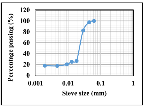
Figs. (1- 4) present the gradation outcomes for fine aggregates, coarse aggregates, bamboo leaf ash, and bagasse ash.
From Fig. (1), the distribution in terms of particle size of the fine aggregate ranges from 0.155 to 4.75mm.The range satisfied the specification of fine aggregate not exceeding 45%, and retained on the sieve based on ASTM – 33 (2003) [46]. Fig. (2) shows the gradation of coarse aggregates. It reveals that the envelope of the curve was within the curve limits as stated according to ASTM – 33 (2003) [46]. Almost 90% of the coarse aggregates fall within 9.5mm to a value of 25mm. Fig. (3) shows the distribution in terms of particle size of the BLA.
From Fig. (3), it can be observed that particles of roughly about 20% lie between 1 µm - 2 µm, and also 80% of these particles lie between 2 µm - 150 µm, conforming to standards of ASTM – D7928 (2017) [54]. This increase the bamboo leaf ash water content and surface area . The particle size for BLA utilised for this study was 150 µm. The particle size distribution of BA is illustrated in Fig. (4). Based on the Fig. (4), approximately 29% of the particles lie within 2 µm - 20 µm. Also, 71% lie between 20 µm -70 µm which conform to the ASTM – D7928 (2017) [54]. As a result, the liquid content as well as the surface area of the baggage ash was raised. The particle size of baggage ash used in this study was 150 µm. The modulus in terms of fineness for the fine aggregate was estimated to be 2.55 and conformed to ASTM -C33- (2003) [46] which stated that fineness modulus should lie between 2.3-3.1.The fine aggregate silt content was found to be 4.67%, conforming to requirements stipulated in ASTM – C33 (2003) [46] which should not exceed 5%. Specific gravity 2.48 and 2.43 of coarse aggregates and fine aggregates met the range stated in ASTM – 33 (2003) [46] between 2.4 – 2.9, respectively. Additionally, the bulk density (rodded) of 1577 kg/m3 and 1495kg/m3 for fine aggregates and coarse aggregates lies between the limit of 1200 - 1750 kg/m3 according to ASTM – C33 (2003) [46] specifications. The water absorption for aggregates was 3.95 and 3.27 which conformed to ASTM – C33 (2003) [46], not reaching beyond 4. The specific gravity of 2.10 and 2.79 for BA and BLA was 33% and 11%, being lower as compared to cement. Furthermore, the bulk density of baggage ash and bamboo leaf ash was about 32% and 33% to that of OPC. The lesser values obtained in reference to bulk density and specific gravity of BA and BLA could lead to a reduction in the density of concrete. The highest particle size of OPC, BA, and BLA was obtained to be 150mm, 90mm, and 150mm, respectively. Table 4 shows the chemical percentages for BA, BLA, and cement.
| Structures | Cement | Coarse Aggregate | Fine Aggregate | BLA | BA |
|---|---|---|---|---|---|
| Specific gravity (bulk) based on SSD | 2.56 | 2.52 | |||
| Specific gravity (bulk) | 3.12 | 2.48 | 2.43 | 2.79 | 2.10 |
| Apparent specific gravity | 2.80 | 2.68 | |||
| Fineness modulus | 2.55 | ||||
| Silt content (%) | 4.67 | ||||
| Water absorption (%) | 3.27 | 3.95 | |||
| Loose bulk density (kg/m3) | 1398 | 1417.5 | 1456 | 365 | 359 |
| Rodded bulk density (kg/m3) | 1435 | 1495 | 1577 | 479 | 471 |
| Voids in loose aggregate (%) | 45.75 | 39.33 | |||
| Voids in rodded aggregate (%) | 39.52 | 34.31 | |||
| Maximum particle size (mm) | 0.09 | 20 | 5 | 0.15 | 0.15 |
| Chemical Anatomy (%) | BLA | BA | Cement |
|---|---|---|---|
| Silica (SiO2) | 69.112 | 70.40 | 20.600 |
| Calcium Oxide (CaO) | 10.814 | 2.90 | 62.927 |
| Aluminium (Al2O3) | 2.523 | 3.54 | 5.985 |
| Iron Oxide (Fe2O3) | 1.741 | 3.93 | 3.341 |
| Phosphorus Oxide (P2O5) | 1.525 | 2.17 | 0.639 |
| Chloride Oxide (Cl) | 0.670 | 0.25 | 0.151 |
| Sulphur Oxide (S) | 0.406 | 0.27 | 2.622 |
| Manganese Oxide (Mn) | 0.245 | 0.20 | 0.129 |
| Potassium Oxide (K2O) | 4.814 | 4.67 | 0.266 |
| Loss of Ignition (LOL) | 8.15 | 11.67 | 3.34 |
The chemical analysis of BA, BLA, and OPC is shown in Table 4. XRD was used to perform the test. According to the results illustrated in Table 4, the percentage of CaO discovered in BLA [55] was higher than BA. However, CaO discovered in cement was larger than BA and BLA. The CaO is the main mechanism behind the establishment of tricalcium silicate and dicalcium silicate which ionises with water to produce about calcium – silicate - hydrate (C-S-H) and it was believed to be the dominant driver in terms of progression of strength. The percentage composition of SiO2 + Al2O3 + Fe2O3 for BA and BLA was found to be 77.87% and 73.38% respectively which exceeded 70% minimum condition based on ASTM C618 (2008) [56] for a pozzolana. Likewise, the LOL of BLA and BA was greater as compared to cement. It fell between the limit of 12% indicated by ASTM C618 (2008) [56]. The physical and chemical features of the superplasticizer adopted in this study are shown in Table 5.
| Attributes | Superplasticizer |
|---|---|
| Coloration | Light brown liquid |
| pH | 5.6 |
| Bulk density (kg/L) | 1.06 |
| Chemical | Polycarboxylate ether |
| Dose | 0.2 – 2% by weight of cement |
4.1. Artificial Neural Network’s Framework Scheme
Three-layer perceptron was constructed through R (nnet package). A total of eleven artificial neural networks were formulated using 214 data sets attained from 27 laboratory concrete mixtures made. The neural network consisted of an input layer, a hidden layer, and an output layer. A total number of 14 input variables (cement, water, BLA, BA, water cement ratio (w/c), fine aggregates, coarse aggregates, aggregate size, curing age, specific gravity coarse, specific gravity fine, fineness modulus, water absorption coarse, water absorption fine) were considered for the analysis. However, curing age, BLA, BA, and cement were the most viable variables employed for the analysis. The compressive strength was the dependent variable. Artificial neural network model independent and dependent characteristics are displayed in Table 6 (Eq. 1).
 |
(1) |
4.2. Training of Neural Network
The 11 neural networks formulated were trained by hidden neurons and activation function. The activation function used for training was linear activation function.
 |
(2) |
Back propagation was utilised for the purpose of networks training. The training process was performed in such a way that, each layer was trained sequentially through forward and backward estimations. The algorithm of the backpropagation consist of two major stages [31].
4.3. Model Efficiency Assessment
The artificial neural network model were trained using a training data set. Testing and validation were performed on testing and validation data set, and degree of precision was computed through the forecasted errors accrued from testing and validation sets. The forecasting accuracy of the ANN model was evaluated using the mean square error (MSE), root mean square error (RMSE), mean absolute error (MAE), mean absolute prediction error (MAPE), and coefficient of determination (R2) by using Eqs. (2-6) accordingly.
| Model Features | Limit | ||||
|---|---|---|---|---|---|
| Minimum | Maximum | ||||
| 1. input factors | |||||
| Water, Kg/m3 | - | 193 | |||
| Cement, Kg/m3 | 312 | 390 | |||
| BLA, Kg/m3 | 19.5 | 78 | |||
| BA, Kg/m3 | 19.5 | 78 | |||
| W/C Ratio, % | - | 0.5 | |||
| Coarse Aggregate, Kg/m3 | - | 993 | |||
| Fine Aggregate, Kg/m3 | - | 662 | |||
| Aggregate Size, mm | 20 | ||||
| Curing Age, days | 28 | 90 | |||
| Specific Gravity Coarse, % | - | 2.56 | |||
| Specific Gravity Fine, % | - | 2.52 | |||
| Fineness Modulus | - | 2.66 | |||
| Water Absorption Coarse, % | - | 3.27 | |||
| Water Absorption Fine, % | - | 3.95 | |||
| 2. Intended Output Parameters | |||||
| Compressive Strength, MPa | 15.8 | 38.5 | |||
 |
(3) |
 |
(4) |
 |
(5) |
 |
(6) |
Where a is the observed value; p is the forecasted value, n represents the concrete sample numbers.
4.4. Feature Relative Importance
Feature importance analysis is performed in order to evaluate the relative impact/significance of input variables on the output of the artificial neural network’s compressive strength forecasting model. The determination of the effect of input parameters on the output is regarded as complex in ANN [28, 57]. In this research, the relative feature importance was performed on the testing and validation data set using R statistical software.
5. ARTIFICIAL NEURAL NETWORK ARCHITECTURE
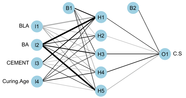
The initial essential phase for establishing an artificial neural network model is ascertaining the ANN architecture. Meanwhile, there is no ground rule for choosing the best artificial neural network architecture, which still requires further study [26, 58]. Thus, following numerous attempts performed, ANN architecture depicted in Fig. (5) was chosen.
The analysis was performed using R (nnet package), and four input variables, five neurons, one hidden layer, and one output were adopted. I 1- I 4 connotes the input variables for the model, B1- B2 stand for bias or threshold introduced during the learning process, H 1- H5 represent the neurons and hidden layer used, and C.S. is the output layer which represents compressive strength. A total of 214 data sets were used. The data sets were divided into two sets and 67% of the data set was used as training set i.e. 144 data while 33% of the data set was used as testing and validation i.e. 70 data. The training, testing and validation data were randomly selected from 28, 56, and 90 days compressive strength values.
5.1. Forecasted Compressive Strength
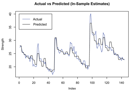
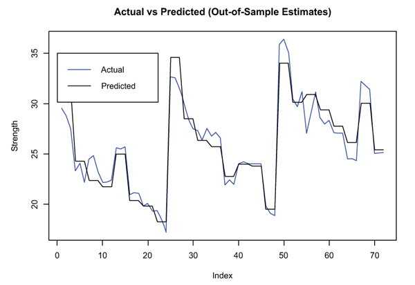
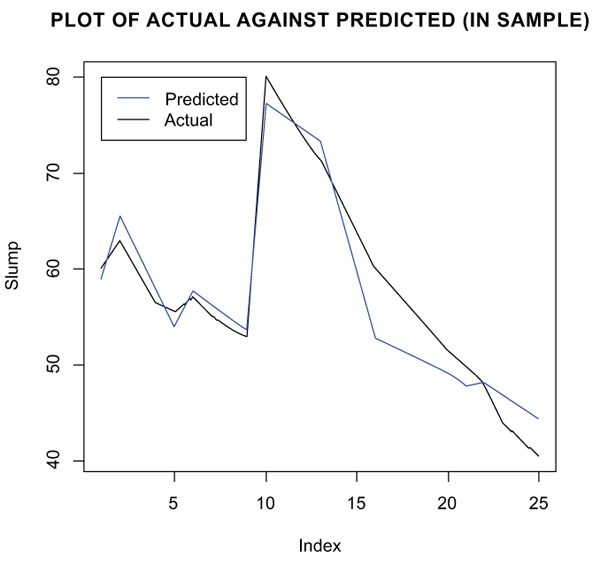
The compressive strength results produced by the model in terms of training, testing and validation were in close range as compared to the actual or experimental values. The visual plots given in Figs. (6 and 7) are the in-sample and out- sample of the actual and predicted values. The effectiveness of the model was assessed through model precision mechanism shown in Tables 7 and 8.
| Model Performance | |||||
|---|---|---|---|---|---|
| Predicted Compressive strength | MAE [MPa] | MSE [MPa] | MAPE [%] | RMSE [MPa] | R2 |
| 0.588 | 0.644 | 2.328 | 0.802 | 0.961 | |
| Model Performance | |||||
|---|---|---|---|---|---|
| Predicted Compressive strength | MAE [MPa] | MSE [MPa] | MAPE [%] | RMSE [MPa] | R2 |
| 1.050 | 1.905 | 3.946 | 1.380 | 0.905 | |
The ANN model’s coefficient of determination for both predicted and actual values for the training was found to be 0.961 while that of testing and validation, it was 0.905. This shows that there is a strong correlation between the actual and predicted values in both the cases. The ANN model forecasted the compressive concrete strength having RMSE of 0.802 MPa for training, while RMSE for testing and validation was 1.380 MPa. This indicated that the differences among the forecasted and actual compressive strength values were negligible in both the cases. The MSE for training was 0.644 MPa and 1.905 MPa for testing and validation, respectively. This signifies that the model over forecasted the compressive strength averagely by 0.644 MPa and 1.905 MPa. The MAE for the training was estimated to be 0.588 MPa which stands for the average difference between the predicted and actual values. The MAE for testing and validation was found to be 1.050 MPa, indicating that, the average difference between the predicted and actual values was minimal. MAPE for the training indicated that the forecasted compressive strength changed averagely by 2.328% from the actual values. While MAPE for testing and validation was 3.946% i.e. the forecasted compressive strength deviated averagely by 3.946% from the actual values. The visual plots shown in Figs. (6 and 7) distinctly display the forecasted compressive strength values which were in close conformity as compared to the actual or experimental values. Its supports that the model has the ability to replicate the actual compressive strength results with great precision.
5.2. Relative Feature Importance Analysis
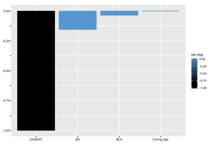
The input features consist of details concerning the expected outputs. Nevertheless, some features might seem to be insignificant which in turn leads to stagnancy in the model. Insignificant features make the training algorithm dummy and noisy. Insignificant features do not impact extra details to the model and can result in deterioration in terms of learning algorithm performance. The relative feature importance of each input feature was built on the testing and validation data set using R statistical software as shown in Fig. (8). The feature relative importance analysis results obtained indicated that curing age is the most significant, followed by bamboo leaf ash (BLA), baggage ash (BA), and cement.
6. MULTIPLE LINEAR REGRESSION
Multiple linear regression (MLR) is a statistical tool which predicts the outcome of a dependent variable using many independent variables. It models the relationship between independent and dependent variables. The analysis was performed using R statistical software. The MLR model was fitted to several independent variables like bamboo leaf ash (BLA), baggage ash (BA), water, cement, coarse aggregate (C.A), fine aggregate (F.A), water binder ratio (W/B), water to solid ratio (W/S), total aggregate –to- binder ratio (TAB), nominal aggregate size (NS), and superplasticizer (SP). Water, C.A, F.A, W/B, TAB, NS and W/S were, however, found to be insignificant.Therefore, the slump data was fitted to only 5 independent variables namely: Cement, BA, BLA, SP1 and SP2. The data was subdivided into two sets. The first 17 values were used as training data and the last 8 values were used as the test and validation data. The MLR model input and output characteristics are shown in Table 7.
| Model Features | Limit | |
|---|---|---|
| 1. Input Variables | Minimum | Maximum |
| Water, W [kg/m3] | - | 195 |
| Cement, C [kg/m3] | 312 | 390 |
| Bamboo Leaf Ash, BLA [kg/m3] | - | 78 |
| Baggash Ash, BA [kg/m3] | - | 78 |
| Coarse aggregates, CA [kg/m3] | - | 993 |
| Fine aggregate, FA [kg/m3] | - | 662 |
| Water to cement ratio, W/C | - | 0.50 |
| superplasticizer | 1.248 | 1.56 |
| Water binder ratio, W/B | - | 0.36 |
| Water to solid ratio, W/S | - | 0.09 |
| Total aggregate –to- binder ratio, TA/B | - | 3.03 |
| Nominal aggregate size, NS [mm] | - | 20 |
| 2. Desired Output Parameters | ||
| Slump [mm] | 40.5 | 80 |
6.1. Best Fitted Slump Model
Out of the 5 independent variables chosen, the best combination of variables that gives the smallest AIC (Akaike information criterion) was chosen as the best model. Step regression was utilised to check the best combination of independent variables that gave the smallest AIC. The results of the step regressions are given in Eqs. (7 and 8).
 |
(7) |
AIC = 44.01
 |
(8) |
AIC = 42.27
From the analysis above, the best model was found to be the one that had Cement, BA, BLA and SP1 as independent variables. The model was fitted and the results are summarized in Table 8. Thus, the fitted model is given in Eq. (9).
 |
(9) |
| Coefficients | Estimate Std. | Error | t value | P-Value |
| (Intercept) | -333.7990 | 50.7215 | -6.581 | 2.61e-05 |
| Cement | 1.0071 | 0.1310 | 7.689 | 5.63e-06 |
| BLA | 0.8365 | 0.1500 | 5.578 | 0.00012 |
| BA | 0.9391 | 0.1171 | 8.019 | 3.67e-06 |
| SP1 | 6.6713 | 2.378 | 2.805 | 0.01591 |
From the P- values in Table 10, it can be seen that all the parameters are significant at 5% level of significance. From the results, we can also see that all the independent variables are positively correlated to slump. Hence, an increase in any of the independent variables would increase the slump value.
6.2. Predicted Slump
The slump results produced by the model in terms of training, testing and validation were very close as compared to that of actual or experimental values based on visual plots given in Figs. (9 and 10). The accuracy of the model was determined by a model precision tool illustrated in Table 9.
| Model performance | |||||
|---|---|---|---|---|---|
| Predicted Slump (training) | Multiple R2 | Adjusted R2 | Residual error | RMSE [mm] | MAPE [%] |
| 0.9336 | 0.9115 | 3.075 | 6.634 | 3.633 | |
| Predicted Slump (testing and validation) | - | - | - | 8.373 | 8.034 |
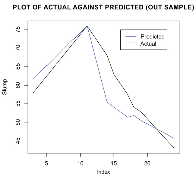
The MLR model’s multiple R2 and adjusted R2 for both predicted and actual values were 0.9336 and 0.9115, which indicated a strong correlation between the actual and predicted values (Table 11). The residual error for the model was estimated to be 3.075 at 12 degrees of freedom. This connotes that the difference between the observed values and forecasted values was not much significant. The MLR model predicted the slump by an RMSE value of 6.634mm for training, while RMSE for testing and validation was 8.373mm. This means that the differences between the predicted and actual slump values were very small. MAPE for the training implies that the forecasted slump values shifted on average by 3.633% from actual data values. MAPE for the testing and validation was 8.034% i.e. the predicted slump changed on average by 8.034% from the actual data. Furthermore, the visual plots illustrated in Fig. (10 and 11) clearly show that the predicted slump values were very close as compared to the experimental or actual values. Therefore, the model has the tendency to duplicate the actual slump results with moderate accuracy.
CONCLUSION
In this paper, multiple linear regression (MLR) and artificial neural network (ANN) were used to forecast the slump and compressive strength of concrete, respectively. The ANN model forecasted the compressive strength for training, testing and validation with a predicted error (RMSE) of 0.802 MPa and 1.380 MPa. The ANN model over forecasted the compressive strength averagely (MSE) by 0.644 MPa for training and 1.905 MPa for testing and validation. The forecasted compressive strength changed averagely (MAPE) by 2.328% for training and 3.946% for testing and validation. The average difference between the forecasted and experimental values (MAE) was 0.588 MPa for training and 1.050 MPa for testing and validation. The coefficient of determination (R2) was 0.961 for training and 0.905 for testing and validation. The curing age, BLA, BA, and cement contributed immensely towards the ANN model output. The MLR model forecasted the slump with predictive error (RMSE) values of 6.634 mm for training and 8.374 mm for testing and validation. The predicted slump deviated (MAPE) averagely by 3.633% for training and 8.034% for testing and validation. The residual error was 3.075 at 12 degrees of freedom. The multiple R2 and adjusted R2 were 0.9336 and 0.9115 respectively. The P-value was found to be 5.639e-07 which is less than 0.05. Hence, the MLR model is a good fit at 5% level of significance. The superplasticizer (SP1+), BLA, BA, and cement contributed greatly towards the MLR model output.
ANN was able to forecast accurately the 28, 56 and 90 days compressive strength. MLR was able to forecast accurately the slump of the concrete. Our work was compared favourably the work of Getahun et al., (2018) at 28 days compressive strength, but the model in this study outperformed their model in terms of 56 and 90 days compressive strength. This is in line with what is found in the literature (compressive strength increases as curing age increases). Comparing the slump result (R2 = 0.9336,RMSE = 6.634) with the result of Yel, 2007 (R2 = 0.8429,RMSE = 9.00), our model performed better.
AUTHORS' CONTRIBUTIONS
O.O; S.M.S. J.M. and A.A. devised the various tests to be performed; O.O. collected the data and executed the experiments ; S.M.S; O.O. J.M. A.A. and C.K. examined the data; S.M.S. dealt with finances; O.O; S.M.S. J.M. A.A. and C.S. prepared the article paper.
CONSENT FOR PUBLICATION
Not applicable.
AVAILABILITY OF DATA AND MATERIALS
The data that support the findings of this study are available from the corresponding author, [O.O., S.M.S., J.M., A.A.A., C.K.], upon request.
FUNDING
This study was supported by The African Union Commission (AUC) and the Japan International Cooperation Agency (JICA) (Grant no. 10.13039 /501100004532).
CONFLICT OF INTEREST
The authors declare no conflict of interest, financial or otherwise.
ACKNOWLEDGEMENTS
Declared none.

