All published articles of this journal are available on ScienceDirect.

A Numerical Study: Transitional Hydrodynamic Behaviour of a Moored Barge in Different Ultra-shallow Water Depths of Malaysia
Authors Info & Affiliations
Abstract
Background:
Malaysia has most of its oil reservoirs in the South China sea. The water depth ranges from 50 m to 200 m. The effects of ultra-shallow water are of prime importance in the exploration of marginal oil fields. Hence, there is an increasing demand for understanding the hydrodynamic behavior of FPSO in ultra-shallow water depths.
Objective:
A simulation study in both frequency-domain and time-domain analyses has been performed to understand the dynamic responses of a moored barge in varying shallow water depths. The objective of this study was to observe the transitional hydrodynamic behavior of the moored barge under varying shallow water depths.
Methods:
The moored barge was administered under regular and irregular waves. Operating conditions for irregular waves in terms of significant wave height and peak time period were incorporated from PETRONAS Technical Standards (PTS). The wave-body interactions and mooring effects have been numerically modelled using a commercial Computational Fluid Dynamics (CFD) and simulation software (ANSYS AQWA) successfully. In order to gain confidence in the simulation software, additional experimental validation was performed for a FPSO model.
Results:
Though the barge was primarily free to rotate in all Degrees Of Freedom (DOF), however, only three DOFs were considered for our study; viz, heave, roll and yaw respectively. The force spectral density, cable RAO’s in addition to the time series of cable forces, along with the effect of significant motions on the mooring cables behavior have been discussed.
Conclusion:
In irregular beam sea state, the significant motions in ultra-shallow water were greater than that for deep waters, this was primarily the main reason for higher cable responses in ultra-shallow water.
1. INTRODUCTION
The oil and gas industries are one of the most lucrative sectors for any nation and overall in a global scenario. The annual global consumption of oil is nearly about 30 billion barrels and continues to increase at a rapid rate. The oil extracted from the earth’s surface also serves as a raw material for various petrochemical and pharmaceutical industries. Hence, the research and explorations of oil and gas, are very important for the nation’s advancement.
With the advancement of technology and monotonous rapid increase in the search of oil fields below water, it has come to extensive exploration in shallow and deep water. Floating Production Storage and Offloading (FPSO) system is fundamentally a floating hull shaped body which is kept in position by mooring lines. The operational depth of water for an FPSO ranges between 50 meters to 1500 meters. The mooring can either be a spread moored system or a turret moored system. Likewise, the concept of FPSO is gaining popularity and at present, there are more than 178 FPSOs located all over the global offshore regions. A recent survey [1] of floating production system offloading revealed that, there are a total of 178 FPSOs working around the globe. 14 FPSOs are currently operating in Australian waters while 51 FPSOs are stationed in Southeast Asia. Malaysia alone has 6 FPSOs.
The remaining part of the paper is organized as follows: Section 2 presents the literature review and past studies related to the hydrodynamics of floating bodies. The numerical modeling of moored barge and mathematical equations related to its analysis are given in Section 3. The details of the laboratory wave tank and equipment are discussed in Section 4 model while Section 5 presents the geometric modeling of the barge along with the mooring layout. The results and discussion of the experimental validation and numerical study are presented in Section 6. Conclusion and remarks are summarized in Section 7.
2. BACKGROUND
Considerable work has been done in station keeping, mooring dynamics, and hydrodynamics of floating structures. The authors in a study [2] have performed a multibody analysis taking into account the hydrodynamic interaction between the FPSO and offloading tanker. The methodology following the decomposition of time-harmonic potential and Green theorem was used to obtain the integral equation. The approach was numerical and experimental, while second and higher orders were neglected in the velocity potential. The research work in another study [3] developed and validated a numerical multibody simulation model for reliable prediction of relative motions and mooring loads during side-by-side operations. They have used Cumin’s equation and a detailed calculation procedure was listed. A CFD program for sloshing analysis with different levels of filling was used in a study [4]. A research study used a mathematical model to predict the second-order responses of FPSO [5]. The approach was numerical. A numerical modeling technique for second-order responses using difference frequency waveform has been illustrated in another study [6]. Using the first-order potential, numerical equations for wave difference second-order force and moments have been discussed. The low-frequency motions for semi-submersible were studied numerically using second-order potential theory in a research study [7]. The second-order force due to incident, radiated and diffracted potential was explained. The authors in another study [8] performed numerical simulations of multiple floating bodies within close proximity in side-by-side offloading configuration. The numerical and mathematical modeling was based on potential theory. Frequency-domain analysis was used to calculate added mass, damping, and other hydrodynamic coefficients. Second-order wave drift forces were also calculated. The research study [9] explained the wave drift damping for horizontal motions only wherein the author performed a numerical and mathematical simulation. Another study [10] described the numerical calculation of the second-order roll moment and compared the obtained results with model tests which were performed for a concept design of FPSO to be operated in severe environmental conditions. The general formulation of second-order wave loads can be obtained by direct integration of the second-order pressure on the hull surface of the body’s mean position, the first-order pressure in the intermittent zone around the waterline and the variation of the first-order loads due to the first-order motions. The near field formulation and middle field formulation were given. The authors in a numerical investigation for the effects of shallow water on multipurpose amphibious vehicle resistance was performed at different speed using CFD [11]. The authors in another study [12], numerically studied the dynamics of liquid sloshing due to uncoupled heave, sway and roll motions. The research study [13] exhibited a numerical and experimental assessment of the second-order responses of a twin-hulled semi-submersible subjected to monochromatic, bi-chromatic and random seas that have been attempted. The wave drift forces in regular waves were obtained using frequency-domain analysis to calculate force linear transfer functions and second-order force component due to second-order temporal acceleration as well as second-order force component due to second-order structural acceleration. The numerical modeling used Weggels Formula and Newmark Beta Method. The authors in another study [14], studied the submarine cable behavior in water during laying operations through a semi-analytical approach. A Higher-Order Boundary Element method (HOBEM) was explained in another research study [15,16], which was used for the computation of the second-order mean wave forces and moments on the ISSC TLP for three different (stationary, freely floating, and tendon-attached) conditions. The direct pressure integration method was used. The research methodology consisted of a higher order boundary element method with greens function. Higher shape functions were used for integration. The prediction of the hydrodynamic performance of FLNG in side-by-side offloading was performed for which potential theory was adopted. Free surface Green's function was used to calculate first-order and second-order forces in frequency-domain. Structural optimization of FPSO availability for bow-to-bow offloading has been studied in another research study [17] and the necessary formulations for equilibrium of FPSO and tanker were given. A research study [18] developed a numerical model for hydrodynamic interaction between two floating bodies in the side-by-side configuration. The study explained the second-order force due to incident, radiated and diffracted potential. The authors in a research study [19] validated second-order forces on floating bodies in regular waves by finite element analysis. The formulation of second-order forces has been explained. The research study [20] presented an experimental study on wave-induced motions on FPSO system in head seas. A green panel method for the dynamics and equations given in WAMIT were used. The authors in another study [21] proposed an estimation method of wind load for the operation of side-by-side offloading including interaction effect of an FLNG and an LNG. The shielding effect of wind was explained. Furthermore, the longitudinal, lateral and yaw coefficient was also explained. Finally, a research work [22] demonstrated that the time-domain numerical simulation of a real system is a good method for determining nonlinear hydrodynamics.
Exhaustive and elaborate studies have been performed in sea keeping and hydrodynamic analysis of FPSOs. Several research works are available on the wave interaction with floating bodies. Malaysia has most of its oil reservoirs in South China Sea where the water depth ranges from 50 m to 200 m. With the above background, the effects of ultra-shallow water are of prime importance in the exploration of marginal oil fields. Hence, there is an increasing demand for understanding the hydrodynamic behavior of FPSO in ultra-shallow water depths. The present study aims at identifying the hydrodynamic behavior of moored barge in different ultra-shallow depths. Initially, a numerical validation was conducted to gain confidence in the numerical software used for studying the dynamics in ultra-shallow water. A real-time simulation and frequency-domain analysis has been performed in numerical software, ‘ANSYS AQWA’ (version 16.2). The hydrodynamic behavior of moored barge was studied for individual heave, roll and yaw excitations only. The significant motions of the moored barge are also post-processed to observe the behavior in six degrees of freedom. The effect of water depths on the mooring cables were explained.
3. METHODOLOGY
3.1. Frequency-domain Hydrodynamic Analysis
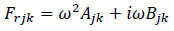
The various fluid forces may be calculated by integrating the pressure over the wetted surface of the body. Fluid forces can be further described in terms of reactive and active components. The active force, or the wave exciting force, is made up of the Froude-Krylov force and the diffraction force. The reactive force is the radiation force due to the radiation waves induced by body motions. The radiation wave potential; ϕrk, may be expressed in real and imaginary parts and substituted to produce the added mass and wave damping coefficients as given in [23,24] (Eqs.1 and 2),
 |
(1) |
 |
(2) |
Where,
Ajk and Bjk are the added mass and damping respectively.
A set of linear algebraic equations were solved in AQWA solver to obtain harmonic response of the body in regular waves. These response characteristics are known as response amplitude operators (RAO) and are proportional to wave amplitude. The set of linear equations of motion with frequency dependent coefficients are given in a study [23],(Eq.3,)
 |
(3) |
Where,
Ms,Ma, C and Khys are the structural mass matrix, added mass matrix, damping matrix and assembled hydrostatic stiffness respectively. (Eq.4)
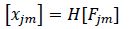
Alternatively,
 |
(4) |
H is the transfer function which relates input forces to output response. The source distribution method was employed in fixed reference axes (FRA). It is assumed that the fluid was ideal such that there would then exist a velocity potential function
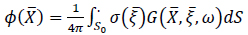
 onto which linear hydrodynamic theory is applied to account for wave radiation and diffraction. Finally, the boundary element integration approach was used to solve the velocity potential function under set of boundary conditions (like kinematic boundary conditions, bottom boundary condition, radiation boundary condition, etc.). In this approach frequency-domain, pulsating boundary condition was introduced in finite water depth given as (Eq.5):
 |
(5) |
Where,
 is the position of source and Dirac-delta function
 is the source strength
G is the Green’s function
The Hess-Smith constant panel method was employed in solver solve the above equation (5), in which the mean wetted surface of a floating body was divided into quadrilateral or triangular panels. It is assumed that the potential and the source strength within each panel were constant and taken as the corresponding average values over that panel surface.
3.2. Real-time-domain Simulation
The simulation solver can generate a time history of the simulated motions of floating structures, arbitrarily connected by articulations or mooring lines, under the action of wind, wave and, current forces. The positions and velocities of the structures were determined at each time step by integrating the accelerations due to these forces in the time-domain, using a two-stage predictor-corrector numerical integration scheme. AQWA-Drift is a module of the solver to simulate the real-time motion of a floating body or bodies while operating in irregular waves. Wave-frequency motions and low period oscillatory drift motions may be considered. Wind and current loading may also be applied. This analysis was used to simulate the real-time motion of a floating body or bodies while operating in irregular waves. Wave-frequency motions and low period oscillatory drift motions can be considered but in the present study, we have solely considered the effect of the waves. The difference-frequency and sum-frequency second-order forces were calculated at each time step in the simulation, together with the first-order wave frequency forces and instantaneous values of all other forces. These are then applied to the structures and the resulting accelerations were calculated, from which the structure positions and velocities are determined at the subsequent time step. The system properties at the end of one-time step are then the starting conditions for the next, and so a time history of the motion of each structure is constructed. The AQWA-Drift analysis is normally applicable for low and moderate sea states. The equation of motion of the floating structure system is expressed in a convolution integral form as given in [23], (Eq.6),
 |
(6) |
Where,
Ma is the fluid added mass, C is the damping including the linear radiation effects, K is the total stiffness matrix, and R is the velocity impulse function matrix.
If the position of center of gravity of structure is defined by
 rotational angle at any time be
 be the wave direction, then the free floating structure RAO based radiation force is given in a study as [24], (Eq.7),
 |
(7) |
Where, m and j are the degrees of freedom, U(wjm,βm) represents the motion RAOs at frequency wjm and relative wave direction (βm) αjm is the normalized mass factor (Eqs.8 and 9).
 |
(8) |
 |
(9) |
The mooring in the present study has been considered as linear elastic cable. It is defined by the stiffness, initial un-stretched length and two attachment points of the mooring line on the linked structures. This line is assumed to have no mass and is therefore represented geometrically by a straight line. Denoting K1 as the mooring line stiffness and L0 as its initial unstretched length, and Pt1 and Pt2 as the attachment points on the two structures (in the fixed reference axes, where one structure may be a fixed location, for instance, an anchor point), the tension on the mooring line is defined (Journee, 2001) (Eq.10).
 |
(10) |
Cable dynamics have been included in our study. When the dynamics of a cable are included in the cable motion analysis, the effects of the cable mass, drag forces, inline elastic tension, and bending moment are considered. Forces on the cable will vary with time, and the cable will generally respond in a nonlinear manner. The solution is fully coupled: the cable tensions and motions of the vessel are mutually interactive, where cables affect vessel motion and vice versa.
The simulation of cable dynamics in AQWA uses a discretization along the cable length and an assembly of the mass and applied/internal forces. In principle, this approach should give the same solution as any of the methods applied in AQWA that have been described previously. However, in the case of a dynamic cable, the inline stiffness is extremely large compared with the transverse stiffness. Besides, the sea bed was modeled with nonlinear springs and dampers, chosen to minimize discontinuities and energy losses at the touchdown point due to the discretization. Forces on each element of the cable were determined and assembled into a symmetric banded global system ready for a solution directly (in the static/frequency-domain) or by integrating in time.
The boundary conditions used in the hydrodynamic analysis are as follows: (Eqs.11-14)
1. Dynamic boundary condition
 |
(11) |
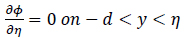
2. Kinematic boundary condition
 |
(12) |
3. Bottom boundary condition
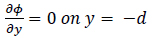 |
(13) |
4. Body surface boundary condition
 |
(14) |
The problem is to solve for the velocity potential ϕ, where ϕ is the sum of incident potential, ϕ0 and scattered potential, ϕs. The incident potential satisfies the boundary value problem mentioned above in the absence of the structure with a change in body surface condition.
5. Radiation boundary condition
The radiation boundary conditions used are shown in Eqs. 15 and 16, respectively.
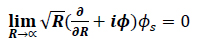 |
(15) |
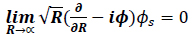 |
(16) |
4. EXPERIMENTAL VALIDATION
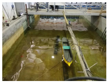
To cite greater confidence of numerical simulation in ANSYS AQWA, an experimental test was carried out in a 22 m long, 10 m wide, and 1.5m deep wave tank in the offshore Laboratory, Universiti Teknologi PETRONAS, Malaysia. The wave tank was fitted with a multi-element HR Wallingford wave maker containing 16 paddles and a wave dissipator. The wave absorber at the other end of the wave tank consists of foam-filled plate fixed to a rigid framework. The wave maker system at UTP offshore laboratory consisted of wave maker, signal generation computer, remote control unit and dynamic wave absorption beach. The wave generator has two modules with each having 8 individual paddles that can move independently to one another. The paddles can move back and forth to create waves in the wave basin. Before starting the model test, all the waves which are intended to be used in the tests were calibrated at the model position. The instantaneous wave elevation was measured using the twin wire wave probes and each time the water depth was changed. Wave probes were calibration and the required water depth was set with free surface set to zero position. During wave calibration, four wave probes were installed. To enable the generation of wave conditions, it is necessary to know the dimensionless Paddle Transfer Function (PTF) which relates the desired wave height upon the model and the associated paddle movement. This relationship is dependent on both water depth and frequency. Hence, it is mandatory to calibrate waves with same wave height and period if they are used at different water depths. For regular waves, the theoretical wave height and wave period are matched with the measured wave height and wave period from the wave probe in the place of model, by adjusting the gain factor in the HR wave maker software.
The wave elevations were measured by twin-wire wave probes. The purposes to perform the measurements are mainly for calibration and means of measuring the details of the wave behavior and hydraulic characteristics of the modeled platform. The probes were attached to the tripod with the probe length 900 mm and diameter 6.0 mm. A simple monitor is equipped with the wave probe to monitor the change of water level during the tests. Each probe shall be calibrated regularly. The calibration was performed by measuring the change in output voltage when the probe is raised or lowered by a known amount in still water. This operation is facilitated by means of a calibrated stem, which is attached to the wave probe and which has a series of accurately spaced holes drilled along its length. Optical tracking system (OptiTrack) is a motion tracking system in 6 DOF that is robust, real-time, and 3D. In this system, it consists of multi-cameras, marker balls, hubs, and calibration tools and keys. To secure high accuracy, the cameras should be arranged so that the views are overlapped and shall be secured firmly in place. This will create a capturing area called capture volume where the tracking will occur. The calibration of the system was performed by using the 3 marker ward, in order to improve the overall performance of the system. Three OptiTrack were used in experimental test. Tension/compression submersible low capacity (250 N) cylindrical shaped and lightweight load cells were used in the test to measure the mooring loads during the tests. Sensors are equipped with 60 m length and 6 mm diameter 4-core shielded chloroprene cable with an output rate of 3000 × 10-6 strain and workable in the temperature range of -20°C to +70°C.
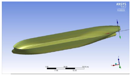
The FPSO model was constructed using wood and 1:100 scale factor was used. Choosing the 1:100 scale allows easy handling of the models as FPSOs are normally having a length in the range of 200 to 300 m. The fabrication was done at the Marine Teknology Lab of UTM Skudai, as they have much experience in fabricating ship and platform models. Additionally, a full scale numerical model was also provided. The model of FPSO is shown in Fig. (1) with the details given in Table (1). The 6 DOF time response was observed for 275 seconds using optical tracking system. Two sets of regular waves were generated for validation study in a water depth of 0.7 m for head sea state. The two sets of regular waves used for experimental validation of FPSO model are shown in Table (2).
5. GEOMETRIC MODELLING OF BARGE AND MOORING LAYOUT
AQWA can simulate linearized hydrodynamic fluid wave loading on floating or fixed rigid bodies. This was accomplished by enforcing three-dimensional radiation/diffraction theory and/or Morison’s equation in regular waves in the frequency-domain. Free-floating hydrostatic and hydrodynamic analyses in the frequency-domain can also be performed. Furthermore, the real-time motion of a floating body or bodies while operating in regular or irregular waves can be simulated, in which nonlinear Froude-Krylov and hydrostatic forces are estimated under the instantaneous incident wave surface. Additionally, the real-time motion of a floating body or bodies while operating in multi-directional or unidirectional irregular waves can be simulated under first- and second-order wave excitations.
Non-linear time-domain simulations were performed to calculate the time series of motion responses for the selected design sea states. Four mooring lines have been used for float-over barge. The anchor mooring lines are modeled as a linear catenary line to ground in the program, and the “hanging” mooring lines are modeled as a hanging catenary line to the fasten structure above water line in the program.
5.1. Hydrodynamic Model
The time-domain (TD) analysis method was used to predict motions and forces during the float-over process. The TD analysis can take into account the nonlinearities in the systems, including the follows:
1. Second-order wave forces and slow drift motions of the barge.
2. Nonlinear forces in the mooring lines.
3. Prior to the time-domain analysis, frequency-domain diffraction/radiation analysis was carried out first to obtain the hydrodynamic coefficients: added mass, wave damping, linear wave forces and mean drift forces.
| Measurement | Model (1:100) | Unit |
|---|---|---|
| LBP | 1.773 | m |
| Beam | 0.3220 | m |
| Depth of hull | 0.259 | m |
| Maximum C/S area | 0.04 | m2 |
| Water plane area | 0.497 | m2 |
The hydrodynamic program was used for the diffraction/radiation analysis. The calculated hydrodynamic coefficients will be used in program ANSYS AQWA for the time-domain analysis. Table 1 displays the geometric details of the moored barge used in the analysis. Fig. (2) is the pictorial representation barge. The focus in these simulations is on the hydrodynamic interactions of spread mooring for the barge. The analysis of the barge was considered with no forward speed. The range of wave direction was varied from -180 degrees to +180 degrees with an interval of 45 degrees leading to 7 numbers of intermediate directions. The range of wave frequency for the hydrodynamic analysis was between 0.05 rad/s to 1.6 rad/s.
5.2. Mooring Details and Layout
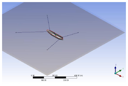
The barge has been moored independently by a horizontal spread mooring system consisting of two lines at the bow and two lines at the stern. The details of the mooring lines for the barge are tabulated below in Table 4. The table also gives the coordinates details of the anchor points as well as the mooring details. The barge was moored in position with four mooring cables. Cable 1 and Cable 2 were connected at the bow of the barge, while Cable 3 and Cable 4 were connected at the aft of the barge. Fig. (3) represents the barge moored in the design modeler of ANSYS AQWA.
6. RESULTS AND DISCUSSION
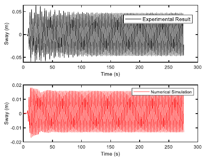
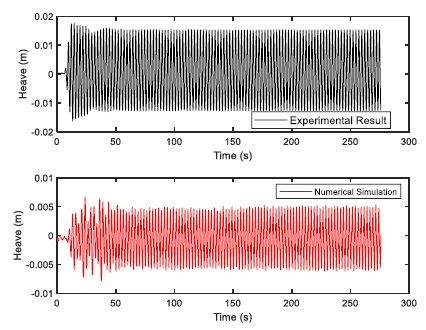
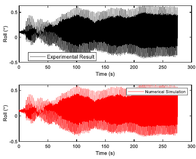
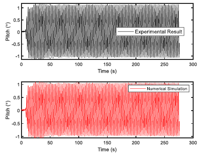
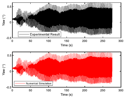
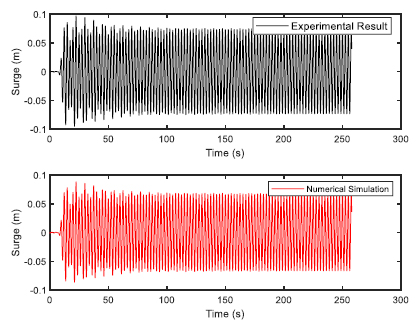
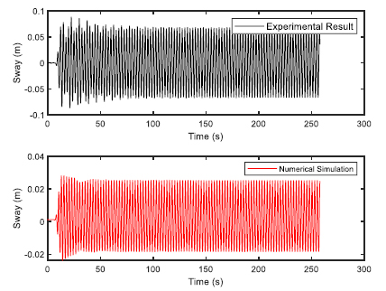
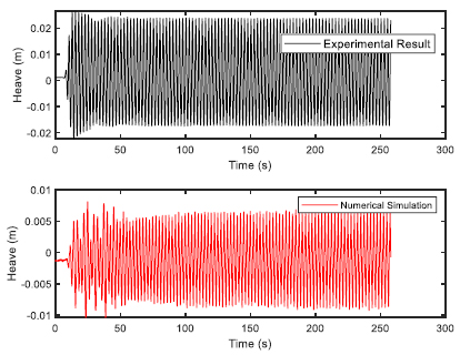
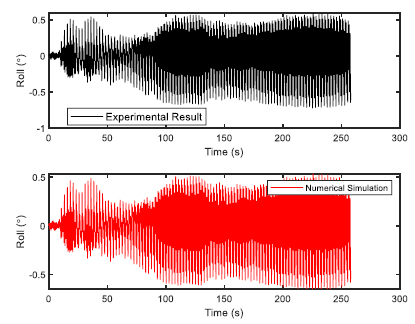
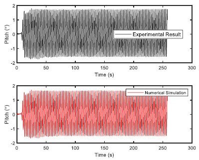
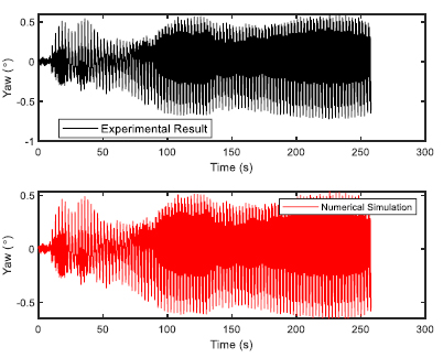
6.1. Experimental Results and Validation
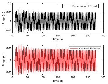
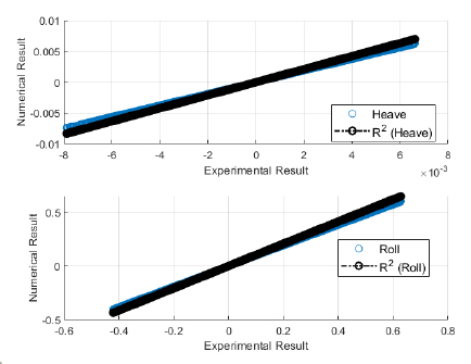
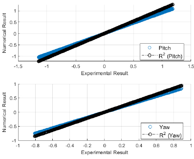
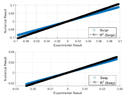
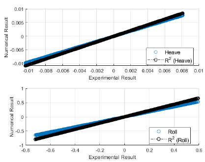
The validation of experimental results with the numerical software are presented here. The validation would build confidence in the simulation and therefore, regression analysis was performed for both the sets of regular waves used in the wave basin. The validation results for first set of regular waves are shown from Figs. (4-9). The validation results for second set of regular waves are displayed from Figs. (10-15).
| Sr. No | Wave Height | Wave Frequency |
|---|---|---|
| 1 | 0.04 m | 0.4 Hz |
| 2 | 0.06 m | 0.4 Hz |
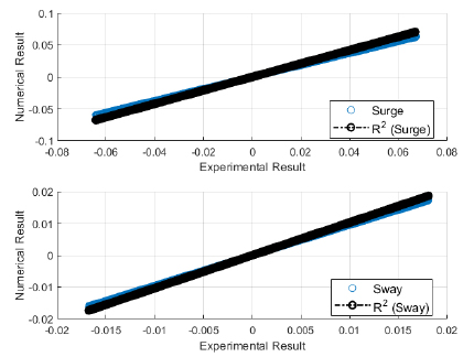
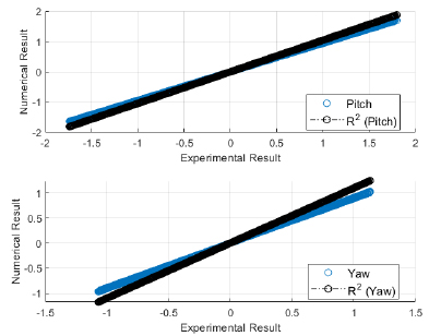
The regression analysis of time motion responses under the two sets of regular waves displayed good agreement between the numerical simulation and experimental lab results. The R-square plot was plotted between the experimental and numerical simulation results for the time response of 6 DOF’s. The R-square plots revealed a good approximation between both tests. The regression result for first set of regular waves are shown from Figs. (16-18) while Figs. (19-21) displays the regression for second set of regular wave, respectively.
6.2. Hydrodynamic Interaction in Regular Waves
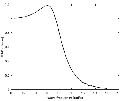
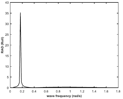
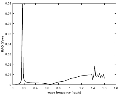
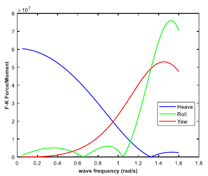
The barge as shown in Fig. (2) was geometrically modeled in the design modeler feature of ANSYS AQWA 16.2, and subjected to hydrodynamic diffraction and response for primarily three shallow water depths. The moored barge was analyzed in regular waves for ultra-shallow water depth of 20 meters solely, while three different water depths as of 20 m, 70 m and 100 m were analyzed for irregular wave conditions respectively. P-M spectrum was used for irregular wave conditions and the corresponding wave data was incorporated from PETRONAS Technical Standards (PTS). The response amplitude operator (RAO) was obtained for the beam sea case. The RAO in three considered directions are plotted in Figs. (22-24), respectively. It was observed that the RAO in heave for beam sea state peaked at 1.18 m/m at a wave frequency of 0.0595 rad/s. The RAO for roll was 35.2 degrees/m, and that for yaw direction was 0.079 degrees/m respectively. Furthermore, the Froude-Krylov forces were plotted in the same considered directions for the regular beam sea condition as shown in Fig. (25). The dominating value of the F-K force was in roll direction, under which the RAO was also maximum.
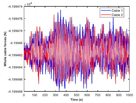
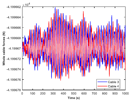
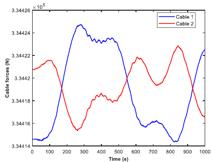
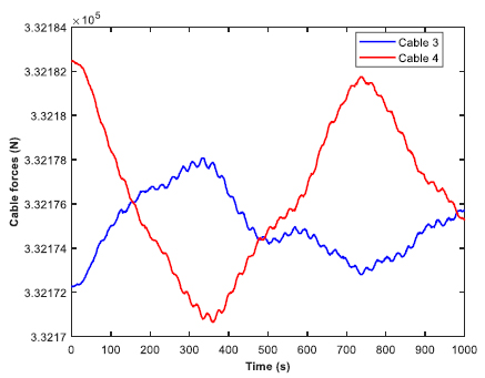
A real time simulation was performed to analyze the cable forces in regular beam sea conditions. The range of time was from 0 to 1000 seconds, with an incremental step of 1 second. All of the four mooring cables were observed, and the time history was plotted for whole cable forces in heave direction. The cable forces were nearly zero in the other two directions (roll and yaw). Moreover, the time history was also plotted for cable forces in tension. The behavior of the mooring cables are depicted in Figs. (26-29), respectively. Two cables were analyzed at a time. There was no significant difference between the values of the forces in cable 1 and cable 2. However, both the cables peaked at different time instants. The similarity in behavior continued between cable 3 and cable 4 as well. The negative values of the forces indicate the tensile nature of force. The peak tension in all the four mooring cables in heave direction were around 41995 N. The whole cable forces were more dominant for the bow positions than the aft position. The bow of the barge is geometrically trimmed and has a comparatively lesser weight and volume. This leads to a heavier aft in terms of weight and volume, compared to the bow. Hence, this supports the claim that the moorings at the bow would require a greater force for the stability of the structure.
6.3. Hydrodynamic Interaction in Irregular Waves
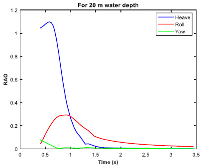
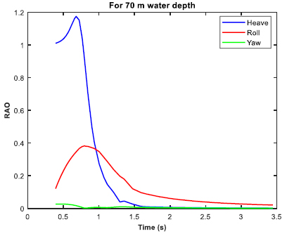
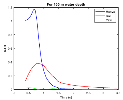
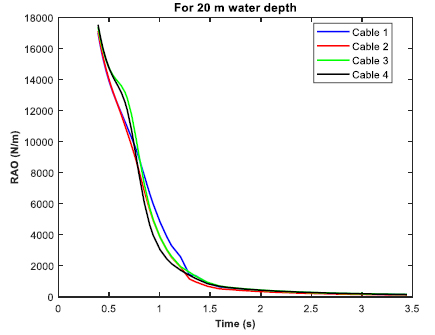
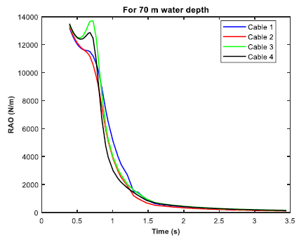
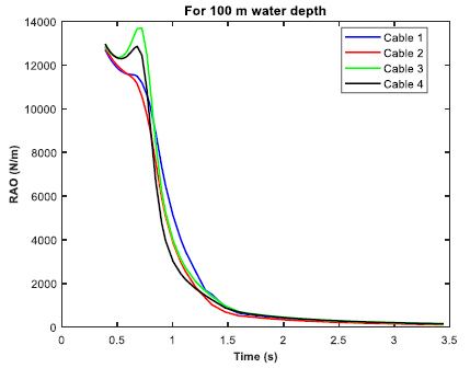
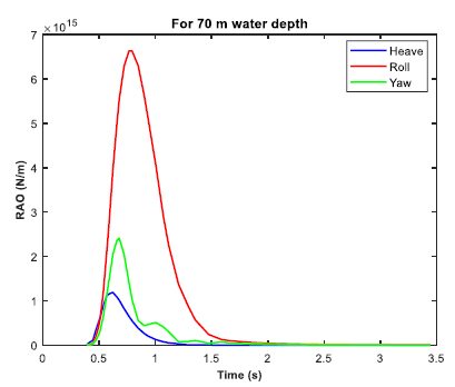
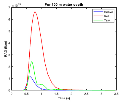
The moored barge was subjected to real time simulation in irregular waves for three different water depths of 20 m, 70 m and 100 m. The P-M spectrum was utilized for the irregular wave analysis. The significant height (Hs) was 3.3 m, and the zero-crossing period (Tz) was 6.7 s. The post processing of the time simulation includes the force/moment spectra in the irregular beam sea, the mooring cable RAO in tension for the irregular beam sea, and the RAO in considered direction (heave, roll and yaw). Figs. (30-32 exhibit the RAO in the irregular beam sea for different ultra-shallow water depths. It is observed that there is a change in the RAO behavior of the barge between 20 and 70 m water depth. However, no significant change in the RAO behavior is observed between 70 m water depth and 100 m water depth as there is not much difference between their depths in comparison to the ultra-shallow depth of 20 m. Table 5 tabulates the summary of the RAO behavior in the three water depths. Figs. (33-35) displays the cable RAO in tension for the three different cases of water depths. It is seen that the profile of the cable RAO between 20 and 70 m water depth had a significant difference, which is not observed between 70 and 100 m water depth. Table 6 tabulates the peak value of cable RAO. Figs. (36-38) are the plots of force/moment spectral density in irregular beam sea, while Table 7 is the summary for the peak values of them.
From the results tabulated in Tables 3-5, it was observed that heave RAO dominates among the three directions, and the peak frequency was more or less the same for varying water depths. However, in ultra-shallow water of 20 m, the heave RAO was initially at a lower value and began to rise as the depth of water increased. For 70 and 100 m water depths, there was no significant difference in the peak values of heave RAO. The RAO in the roll and yaw mode of freedom had little variation and the value is also considerably less. With due consideration to the Cable tension RAO, the shallow water at the minimum depth had the highest RAO, while the amount tended to reduce as the depth of water increased. It can be construed that cable responses were higher in shallow depth and tends to reduce as the water depth increases. The roll spectral moment was seen to be dominating and its value gradually increased as water depth increased. The peak frequency responsible for the roll spectral moment was almost the same in all the three cases of water depth.

| Details of Point Mass (Inertia Values Defined by Radius of Gyration) | |
|---|---|
| Mass | 45172366.601 kg |
| Kxx | 13.6 m |
| Kyy | 50 m |
| Kzz | 52 m |
| Ixx | 8355080926.625 kg.m² |
| Iyy | 112930916503.906 kg.m² |
| Izz | 122146079290.625 kg.m² |
| Details of Mesh | |
| Tolerance | 0.2 m |
| Maximum element size | 0.8 m |
| Maximum allowed frequency | 8.234 rad/s |
| Number of nodes | 13450 |
| Number of elements | 13348 |
| Number of diffracting nodes | 7854 |
| Number of diffracting elements | 7729 |
| Details of Wave Directions | |
| Wave Range | -180° to 180° |
| Interval | 45° |
| Number of intermediate directions | 7 |
| Specification | Details of Geometry |
|---|---|
| Connection Point 1 | (20,14.2,8) m |
| Connection Point 2 | (20,-14.2,8) m |
| Connection Point 3 | (180,16,8) m |
| Connection Point 4 | (180,-16,8) m |
| Anchor 1 | (-200,200,-20) m |
| Anchor 2 | (-200,-200,-20) m |
| Anchor 3 | (200,200,-20) m |
| Anchor 4 | (200,-200,-20) m |
| Mass/Unit Length | 150 kg/m |
| Equivalent Cross-Sectional Area | 0.01 m² |
| Stiffness, EA | 600000000 N |
| Maximum Tension | 7500000 N |
| Water Depth | Heave | Roll | Yaw | |||
|---|---|---|---|---|---|---|
| Peak Max (m/m) |
Frequency (rad/s) | Peak Max (degree/m) | Frequency (rad/s) | Peak Max (degree/m) | Frequency (rad/s) | |
| 20 m | 1.098 | 0.586 | 0.292 | 0.936 | 0.078 | 0.391 |
| 70 m | 1.175 | 0.679 | 0.382 | 0.793 | 0.026 | 0.469 |
| 100 m | 1.174 | 0.679 | 0.382 | 0.793 | 0.025 | 0.509 |
| Cable Profile/Water Depth | 20 m | 70 m | 100 m | |||
|---|---|---|---|---|---|---|
| Peak Max (N/m) | Frequency (rad/s) | Peak Max (N/m) | Frequency (rad/s) | Peak Max (N/m) | Frequency (rad/s) | |
| Cable 1 | 17006.05 | 0.391 | 13216.901 | 0.391 | 12704.98 | 0.391 |
| Cable 2 | 17132.768 | 0.391 | 13328.093 | 0.391 | 12818.117 | 0.391 |
| Cable 3 | 17377.088 | 0.391 | 13698.774 | 0.722 | 13691.249 | 0.722 |
| Cable 4 | 17534.715 | 0.391 | 13497.972 | 0.391 | 12967.665 | 0.391 |
| Water Depth | Heave | Roll | Yaw | |||
|---|---|---|---|---|---|---|
| Peak Max (N²/(rad/s)) |
Freq. (rad/s) | Peak Max ((N.m)²/(rad/s)) | Freq. (rad/s) | Peak Max ((N.m)²/(rad/s)) | Freq. (rad/s) | |
| 20 m | 1.8855E+15 | 0.621 | 4.1598E+15 | 0.793 | 3.7586E+15 | 0.621 |
| 70 m | 1.1853E+15 | 0.621 | 6.6326E+15 | 0.765 | 2.4060E+15 | 0.679 |
| 100 m | 1.1561E+15 | 0.621 | 6.6206E+15 | 0.793 | 2.4351E+15 | 0.621 |
| Significant Motions (20 m water depth) | Significant Motions (70 m water depth) | Significant Motions (100 m water depth) | |
|---|---|---|---|
| Surge (X) | 3.0973E-02 m | 2.7701E-02 m | 2.7834E-02 m |
| Sway (Y) | 0.9713 m | 0.8125 m | 0.8046 m |
| Heave (Z) | 1.2964 m | 1.4308 m | 1.4294 m |
| Roll (RX) | 0.3929° | 0.5297° | 0.5309° |
| Pitch (RY) | 0.1928° | 0.1926° | 0.1925° |
| Yaw (RZ) | 3.6318E-02° | 2.3887E-02° | 2.3684E-02° |
The data in Table 8 shows the significant motion of the moored barge in the three different water depths, it was observed that for the ultra-shallow depth of 20 m; there was a considerable amount of heave, roll, and sway. But as the water depth increased to 70 m, the sway motion reduced by 16%, and further for 100 m water depth the sway motion nearly reduced to 17% from the initial. Whereas, the value of heave motion increased by 10% of the value at the 20 m depth of water. Similarly, the roll motion increased by 35% as the water depth increased from 20 to 100 m. It was further observed that the motion responses were significant in shallow water and as and when the water depth increased, the motion in the surge direction, sway direction, pitch direction, and yaw direction continued to decrease while giving an increase in the heave and roll motion only. Thus, the reason for the reduction in cable tension as the water depth increases is primarily because of the reduction in the significant motions of the moored barge.
CONCLUSION
There was a good validation between the experimental results and the numerical simulation. The hydrodynamic wave interaction and real time simulation analysis on the floating moored barge was investigated. From the obtained results and comparisons with the simulations under the different water depths, the following conclusions may be drawn.
1. In the regular beam sea, the RAO was higher in the heave direction for a lower value of frequency, but roll response was higher for the Froude-Krylov forces on the moored barge, peaking at higher wave frequency.
2. In the regular beam sea, whole cable forces were present in the heave direction but these were zero for roll and yaw motions.
3. In a regular beam sea, the mooring cables depicted similar behavior, but each one of them peaked at different time intervals. However, the cable forces in tension were dominant for those cables at the bow positions due to the shape of the barge.
4. In the irregular beam sea, the response is higher in ultra-shallow water, and this gradually reduced in increasing water depths.
5. In irregular beam sea, the response for mooring cables was also seen to dominate in ultra-shallow water, while their response was considerably lower as water depth increased.
6. In irregular beam sea, there were more significant motions in the ultra-shallow water than that for deep water depth. This was primarily the main reason for a higher cable response in ultra-shallow water.
As a part of future work, operability, and downtime cost analysis would be studied for the offloading operations.
NOMENCLATURE
| ϕrk | = Radiation wave potential |
| ϕ | = Velocity potential |
| P | = Density |
| w | = wave frequency |
| we | = encountering wave frequency |
| X | = wave direction |
| δ | = source strength |
| βm | = Relative wave direction |
| T | = Tension |
| αm | = Normalized mass factor |
CONSENT FOR PUBLICATION
Not applicable.
AVAILABILITY OF DATA AND MATERIALS
The author confirms that the data supporting the findings of this study are available within the article.
FUNDING
This project has been funded by YUTP grant (Cost center: 015LCO-095).
CONFLICT OF INTEREST
The author declares no conflict of interest, financial or otherwise.
ACKNOWLEDGEMENTS
The support and encouragement provided by the Universiti Teknologi PETRONAS (UTP) and Curtin University (Perth) are gratefully acknowledged. This project has been funded by YUTP grant (Cost center: 015LCO-095).