All published articles of this journal are available on ScienceDirect.

Guidelines for Geotechnical Finite-Element Modeling
Abstract
This paper emphasizes on the required guidelines for establishing a geotechnical finite-element model. The steps that must be taken to construct such a model are explained in a flowchart, and the methodology described therein is illustrated by building a model using commercially available finite-element software. Well-documented experimental test data are used to validate the model results. The effects of the geometry plotting, meshing techniques, and boundary locations are assessed by comparing the model results with the experimental results. To date, various geotechnical constitutive models have been proposed to describe various aspects of actual soil behavior in detail, and the advantages and limitations of five such models are discussed. The model results are subjected to an assessment check. The geotechnical modeler can be decided based on the knowledge base that constitutive models will use as the case.
1. INTRODUCTION
In geotechnical engineering, the frequently used term “Finite-Element (FE) modeling” refers to a numerical technique whereby engineering structures and their surrounding soil are discretized into certain numerical elements that obey specific constitutive laws. Because soil behaves in a complicated and nonlinear manner, all methods for modeling it are necessarily numerical [1], and geotechnical engineers tend to use methods based on FE theory. A numerical FE model of a geotechnical problem must simulate the actual field conditions of that problem. The model must capture the complex behavior of the soil to provide accurate deformations, settlement, and straining actions, thereby giving engineers a unique perspective for making evaluations and judgments.
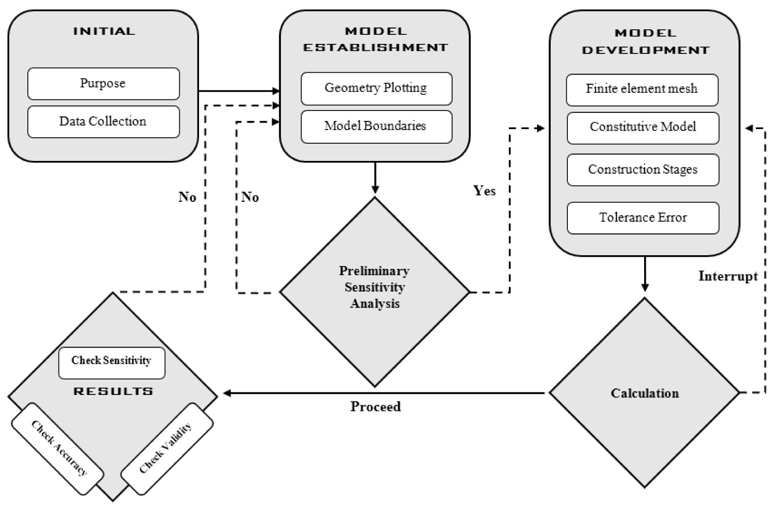
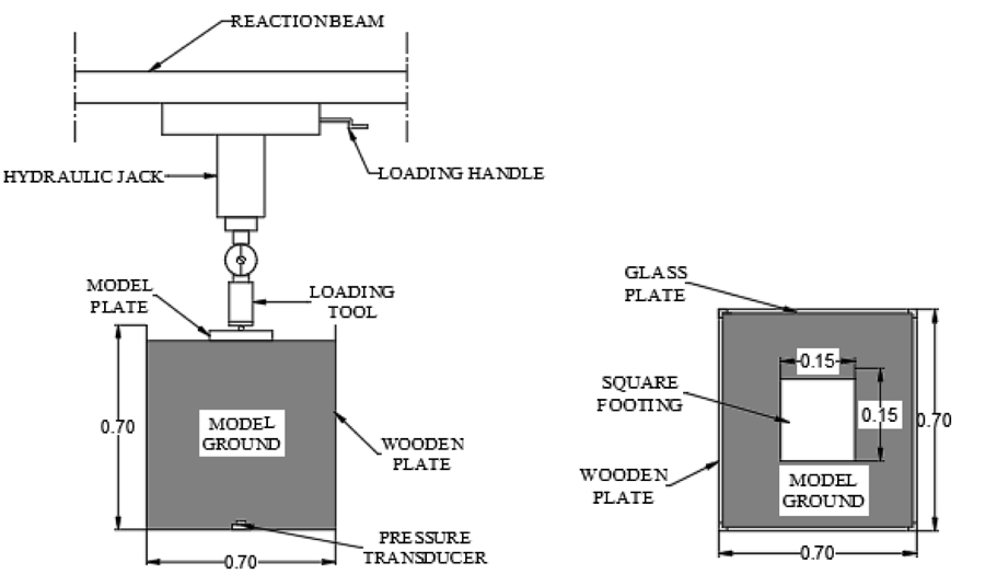
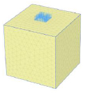
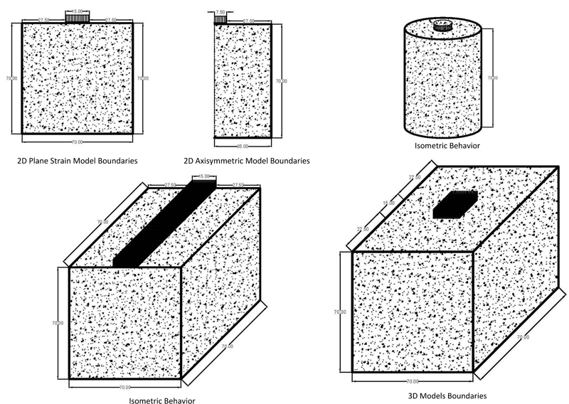
Fig. (1) shows a flowchart that explains the stages of establishing a geotechnical FE model. To explain the modeling stages easily, each stage is illustrated using a selected case study. A study carried out laboratory experiments to provide data to verify associated two-dimensional (2D) and three-dimensional (3D) FE models [2]. This work involved measuring the vertical stress under a square footing of 0.15 m × 0.15 m acting on a sample of sandy soil with 0.70 m × 0.70 m × 0.70 m, as shown in Fig. (2). The main stages of the FE example model are summarized in Table 1.
In the study mentioned [2], the main purpose of the FE models was to measure the vertical stress occurring under the centerline of the uniformly loaded square footing at specific depths. An additional goal after verifying the model was to use it to investigate the expected settlement trough.
2. INITIAL STAGE OF MODELING
2.1. Purpose of Model
The first step in establishing an FE model is to identify the purpose of the analysis. The model may be intended for (i) structural failure prediction, (ii) deformation determination, (iii) consolidation analysis, or (iv) water flow analysis, among others. Each of the above stage needs a specific approach; therefore, the aim must be defined at the outset.
2.2. Data Collection
After defining the model's primary purpose, an extensive search is required for information sources and site investigations. The required information comes in the following four main categories.
2.2.1. Ground Geotechnical Information
The ground investigation must be planned carefully to get the information needed to represent the ground materials in the FE model accurately. The site conditions are defined mainly from characterization tests and borehole sampling descriptions. Depending on the purpose of the analysis, the essential geotechnical parameter values can be determined from specialized parameter testing.
In the selected case study [2], the tested soil stratum was defined according to the Unified Soil Classification System. The tested sand was poorly graded sand (SP); the index properties are listed in Table 2. The geotechnical parameters take the measured values, except for the cohesion, which was changed from zero to 1.00 kN/m2 to avoid numerical error calculations.
| S.No | Stage | Sub-Stages | Description |
|---|---|---|---|
| 1 | Initial | Purpose | Measure vertical stress occurring at the centerline of uniformly loaded square footing at specific depths and determine the settlement trough |
| Data collection | Collect geotechnical information (Table 2) | ||
| 2 | Model establishment | Geometry plotting | Geometries (Table 3) and graphs (Figs. 3 and 4) of three FE models |
| Model boundaries | Boundary dimensions of the three FE models (Fig. 4) | ||
| 3 | Model development | Meshing | A graded mesh (Fig. 7) |
| Constitutive models | Choose the Mohr-Coulomb and linear elastic constitutive models (Figs. 3 and 4) | ||
| Construction stages | In the initial stage, K0 analysis is used. In the construction phases, plastic analysis is used. No water pressure analysis was performed. | ||
| Tolerance error | Force criterion used as a stopping criterion with a tolerance of 0.01 | ||
| 4 | Results | Check sensitivity | Boundary conditions checked with almost zero deformation on the edges |
| Check validity | Results validated using the laboratory results of Keskin et al. (2008) | ||
| Check accuracy | Calculated errors in final results: • Axisymmetric: (25.29±2)% • Plain strain: (90.40±22)% • 3D: (11.01±2)% |
| Parameter | Value | Unit |
|---|---|---|
| Relative density (Dr) | 65.00 | % |
| Dry unit weight (γdry) | 17.10 | kN/m3 |
| Young’s modulus (E) | 28 000 | kN/m2 |
| Cohesion (c) | 0.0 | kN/m2 |
| Internal friction angle (φ) | 41.00 | ° |
| Dilatation angle (ψ) | 11.00 | ° |
| Poisson’s ratio (ν) | 0.20 | - |
| Technique | 2D Plane Strain | 2D Axisymmetric | 3D |
|---|---|---|---|
| Definition | To analyze a vertical plane section through the site. In the third dimension (i.e., perpendicular to the plane), strain and displacement are assumed to be zero. |
Except that one vertical side of the plane (often the left-hand side) is the axis around which the site exhibits rotational symmetry, analysis of plane, i.e., vertical section across the site, must be conducted. The radius from the axis of symmetry is the horizontal axis, and the strain perpendicular to the plane and in the circumferential or hoop direction is considered to be zero. | Analysis using three dimensions considering the full-scale model |
| Applications | Suitable to sites with a uniform cross-section, including ground conditions (ii) stress state/loading for a sufficiently long straight dimension for virtually zero strain to be expected in the long dimension (e.g., straight tunnels, embankments, long excavations, strip foundations). | Suitable for sites with a vertical structure in the ground with a uniform radial cross-section (e.g., vertical shaft, circular cofferdam, single vertical pile, circular spread foundation) and vertical loading that is uniform around the central axis. | Suited to all cases and site conditions |
| Limitations | Sites with pile foundations, ground anchors, or similar structural geometries are not suitable. | Suited to structures with a radial cross-section only | Time-consuming and requires considerable computational power |
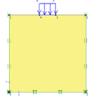
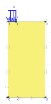
| Model configuration |
|
|
|
2.2.2. Geological Information
Data from geological surveys are crucial for determining the values of specific ground parameters, especially regarding rock mechanics. However, no geological information is required in the present case.
2.2.3. Historical Information and Construction Stages
The stress history and stress path have considerable effects on the behavior of soil and rocks. The historical construction stages up to the present day must be simulated in the FE model if the simulation of the stress path and current stress state is accurate.
3. MODEL ESTABLISHMENT
3.1. Geometry Plotting
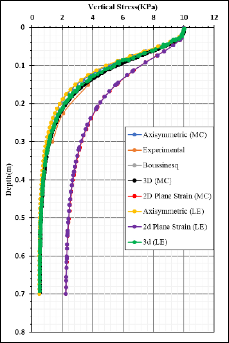
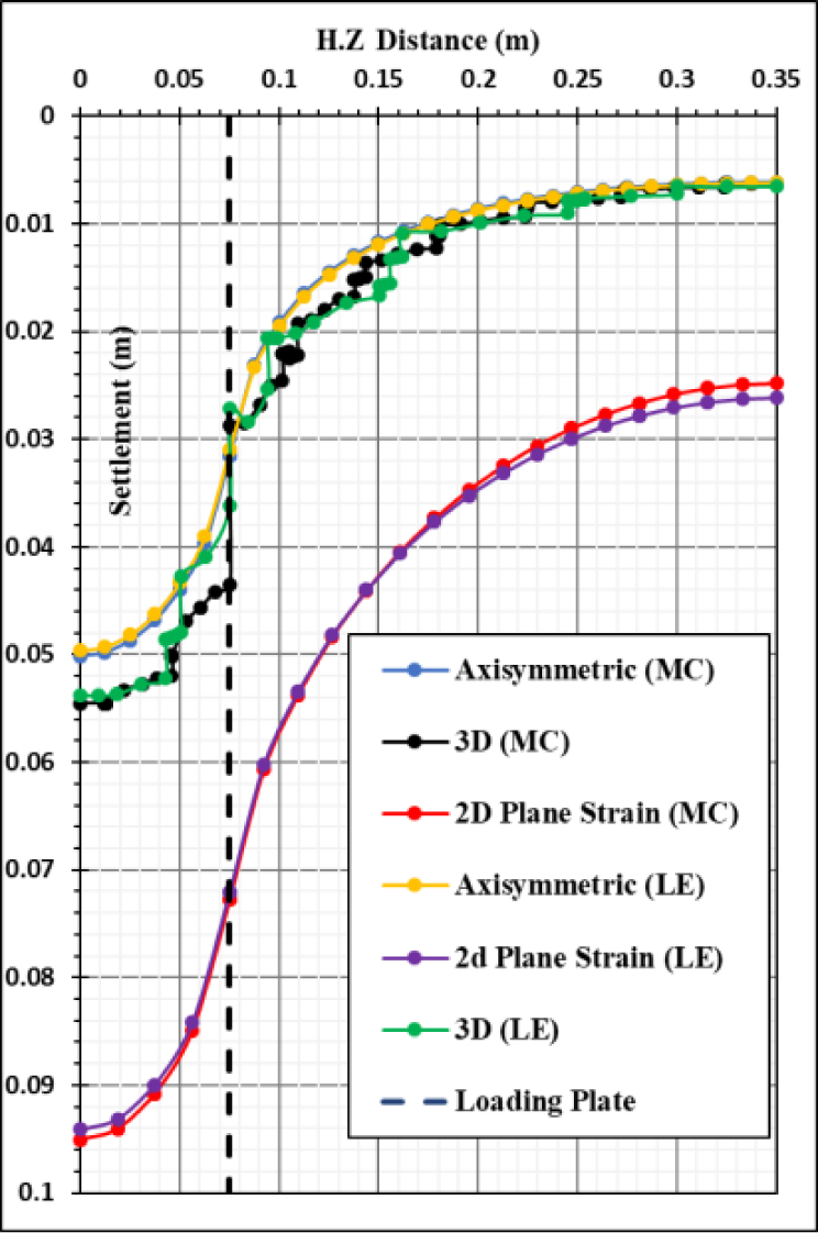
Three FE models are established and plotted, namely (i) a 2D plane strain model, (ii) a 2D axisymmetric model, and (iii) a 3D model, of which the 3D model is the most realistic for the square loading plate. The 2D axisymmetric model treats the footing as circular rather than square, giving an acceptable error in the desired results. The 2D plane strain model is the least suited to the present geometry, treating the square loading plate as rectangular with dimensions of 0.15 mm × 1.00 mm, exhibiting a significant error in the results. Table 3 describes the different techniques of geometry plotting. The results of the case study are described graphically in Figs. (3 and 4). Fig. (3) shows the vertical stress versus depth, and Fig. (4) shows the settlement trough in a plot of settlement versus horizontal distance from the center of the footing.
3.2. Model Boundaries
3.2.1. Location
The FE mesh must be fixed in space to determine the displacement to solve the global stiffness equation. The fixedness is applied at the model's boundaries; however, there are often no defined boundaries for the FE model because the ground extends indefinitely. As a result, some judgment is necessary when choosing where the model borders should be placed. The borders should not be set too near the region of interest since this would be impractical and result in a strong boundary effect. The fixedness imposed at the boundaries would begin to impact the critical outputs.
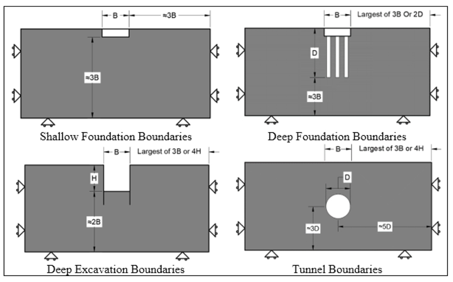
For the selected case study, the dimensions of the laboratory model provide clearly defined boundaries, as shown in Fig. (5). The boundaries should not be placed too close to the area of interest because that would be unrealistic and introduce a significant boundary effect, i.e., the fixedness imposed at the boundaries would start to influence the key outputs. The boundaries affect the FE meshing, and a sensitivity analysis is crucial for determining the appropriate boundaries. Fig. (6) shows the expected boundaries for different cases.
3.2.2. Types of Fixedness at Model Boundaries
The standard types of fixedness applied at the model boundaries are (i) zero displacement in all directions at the bottom boundary and (ii) zero displacement on the vertical sides in the horizontal direction perpendicular to all those boundaries, including on axes of symmetry. The top surface has no fixedness imposed.
The nature of the fixedness is minor at faraway model borders that are sufficiently far from the region of interest. Indeed, varying such fixedness provides a way to assess the sensitivity of the essential outputs to boundary effects.
4. MODEL DEVELOPMENT
4.1. Meshing
After the model's geometry has been created, it is replaced with an equal FE mesh that uses continuum elements to represent the ground. Elements generate the mesh based on the degree of precision necessary in the model (a higher number of minor elements gives great precision). The nodes, which are discrete places where the significant unknowns (displacement or excess pore pressure) are computed, link the components. Shape functions or interpolation functions are used to interpolate nodal displacements for all points in each element to yield secondary or derived quantities of strains or strain rates, as well as stresses or stress rates. The stresses and strains are computed at Gauss, stress, or integration points located across the element.
4.1.1. Types of Element
Higher-order elements contain more nodes and Gauss points, resulting in more precise stress computations, especially stiff behavior. In geotechnical FE analysis, linear and cubic strain element types are widely employed. Linear strain elements are quick to compute and are adequate for most deformation studies if there are enough of them. They might not be appropriate for 2D axisymmetric models, and they might overestimate failure loads in all models (although this tendency is reduced by using reduced integration).
To forecast failure situations in general, and in particular, for axisymmetric models, cubic strain elements (e.g., a 15-node triangle) are favored despite the associated slower computation. When analyzing groundwater flow, lower-order elements are appropriate or even preferred in some programs. The triangular (2D) and tetrahedral (3D) elements have the advantages of I fitting into complex forms more readily, (ii) being compatible with automatic mesh generators, and (iii) being less prone to distortion mistakes. Element definition begins by assuming a displacement field caused by a shape function such as a one-dimensional, 2D, or 3D element. Table 4 shows the hierarchy of element categories.
| Shape Function | Variation Across Element | Elements for Continua | |
|---|---|---|---|
| Displacement | Strain | ||
| First-order | Linear | Constant | TRI3, QUAD4, TET4, HEX8 |
| Second-order | Quadratic | Linear | TRI6, QUAD9, TET10, HEX20 |
| Third-order | Cubic | Quadratic | TRI10, QUAD16, |
| Fourth-order | Quartic | Cubic | TRI5 |
4.1.2. Interface Elements
Interface elements are used to create a relative displacement between elements in the normal and shear directions. There are two types of interfaces, namely a line interface and a plane interface. A line interface is used between two planar elements (plane stress or plane strain) or between planar elements and structural elements (beam and truss elements); it consists of either 4- or 6-node elements. A plane interface is used between two solid elements or between solid and planar elements; it consists of either 6- or 12-node elements for triangular elements and 8- or 16-node elements for rectangular elements. Overall, increasing the number of nodes in a specific element captures more of the actual soil behavior. The only constraints are the available computing power and analysis time.
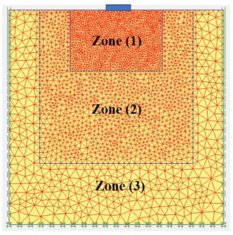
4.1.3. Mesh Size
The most precise mesh would be one with small elements all over, but this would take a long time to compute. A good FE mesh is graded, with minor components just where needed and more significant elements far away from the area of concern, where stresses and strains are more evenly distributed. Fig. (7) shows the mesh used in the present case. Zone 1 is the area of interest with the minor elements, zone 2 is farther away with intermediate-size elements, and zone 3 is the farthest away with the most considerable elements. Such a mesh offers faster computation with no significant loss of accuracy.
Because of the larger number of nodes per element, meshes made with higher-order elements can be coarser. Higher-order elements heavily influence the prediction of collapse loads, and meshes make those elements progressively finer until collapse loads appear unaffected by mesh geometry. The displacement and stress distributions computed by the interpolation functions are only reliable if the element shapes are not altered significantly.
Due to the inability of automatic mesh generators to control such distortion, it must be verified manually. If the sides of each element are about the same length, distortion is less of an issue for triangular and tetrahedral elements.
4.2. Material Constitutive Models
Table 5 describes the most common constitutive models used to represent ground behavior. In the present case study, the results obtained with the linear elastic (LE) and Mohr-Coulomb (MC) constitutive models are plotted in (Figs. 3 and 4), showing minor differences.
4.3. Construction
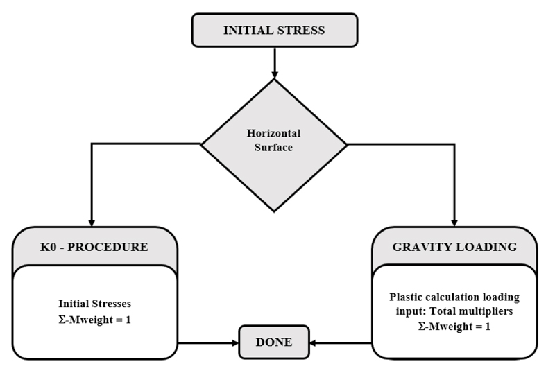
4.3.1. Initial Stresses
In terms of FE modeling, any nonlinear constitutive model's predicted stress-strain behavior is dependent on the current stress state. When material properties are dependent on whether the material is above or below the groundwater level, the groundwater level should coincide with element boundaries. Once the pore pressure profile and ground densities are known, the effective vertical stress is relatively simple to calculate; however, the effective horizontal stress must be calculated from the vertical stress using the stress ratio K0.
Many approximate equations are available to help validate measured values or estimate K0, such as Jaky’s equation [11] used for customarily consolidated soils. For overconsolidated soils, other more approximate equations have been proposed for estimating K0 [12]. As shown in Fig. (8), there are two methods for determining the initial stress in a FE analysis. Direct specification (K0 method) is used for homogeneous stress profiles with a horizontal ground surface, strata, and groundwater levels. Because the FE analysis achieves vertical equilibrium while the horizontal stress is based solely on the specified K0 or horizontal stress values, the equilibrium may not be achieved. Minor equilibrium errors may be acceptable due to a slight inclination in the layers or ground surface. In this case, a plastic nil-step should be performed after the initial stress is established.
| Model | Definition | Parameters | Applications | Limitations |
|---|---|---|---|---|
| Mohr-Coulomb (MC) | A well-known and straightforward linear elastic-plastic model that offers first approximation of soil behavior. The linear elastic part of the MC model is based on Hooke’s law of isotropic elasticity. The perfectly plastic part is based on the MC failure criterion, formulated in a non-associated plasticity framework. |
E [kN/m2]: Young’s modulus υur: Poisson’s ratio c [kN/m2]: cohesion φ [°]: friction angle Ψ [°]: dilatancy angle |
•Used to model soil behavior in general •Failure behavior is generally well captured (at least for drained conditions) •Can provide the first estimate of deformation |
•Has limited ability to model deformation behavior accurately before failure, especially when stress level changes significantly or multiple different stress paths are followed •When used for excavation and retaining-wall problems, it generally leads to a massive pit bottom heave, which may cause an unrealistic uplift of the retaining wall •In tunneling problems, its use produces a settlement trough that is generally too wide |
| Linear Elastic (LE) | It obeys Hooke’s law of linear relation between stress and strain. Materials modeled using the LE model are deformed elastically throughout the analysis, which means that they return to their initial state upon unloading. |
E [kN/m2]: Young’s modulus υur: Poisson’s ratio |
Used to model stiff materials in soil (e.g., thick concrete walls or plates, rock layers) or far-field areas where plasticity plays no significant role. | •Not suitable for modeling soil in general •Cannot estimate failure behavior |
| Hardening Soil (HS) | A true second-order model for soils in general (soft soils and harder ones) for any application. Involves friction hardening to model plastic shear strain in deviatoric loading and cap hardening to model plastic volumetric strain in primary compression. |
c [kN/m2]: cohesion φ [°]: friction angle Ψ [°]: dilatancy angle St [kN/m2]: tension cut-off and tensile strength E50ref [kN/m2]: secant stiffness in standard drained triaxial test EOedref [kN/m2]: tangent stiffness for primary oedometer loading Eurref [kN/m2]: unloading/reloading stiffness m: Power of stress-level dependency on stiffness |
•Accurate for problems involving a reduction of mean effective stress and, at the same time, mobilization of shear strength. Such situations occur in excavations (retaining-wall problems) and tunnel construction projects •It can be used to predict displacement and failure accurately for general types of soil in various geotechnical applications |
•It does not include anisotropic strength or stiffness, nor time-dependent behavior (creep) •Has limited ability for dynamic applications |
| Hoek–Brown (HB) | An empirically derived relationship is used to describe a nonlinear increase in peak strength of isotropic rock with increasing confining stress. It follows a nonlinear, parabolic form that distinguishes it from the linear MC failure criterion. Includes companion procedures developed to provide a practical means to estimate rock mass strength from laboratory test values and field observations. |
Erm [kN/m2]: rock-mass Young’s modulus υ: Poisson’s ratio Sci [kN/m2]: uniaxial compressive strength of intact rock mi: intact-rock parameter GSI: geological strength index Ψmax [°]: dilatancy angle (at s′3=0) SΨ [kN/m2]: an absolute value of confining pressure s′3 at which Ψ=0 |
•Nonlinear in form (in the meridian plane), which agrees with experimental data over a range of confining stress •Developed through an extensive evaluation of laboratory test data covering a wide range of intact rocks •Provides a straightforward empirical means to estimate rock-mass properties |
•Limitations documented in detailed discussions on the simplifying assumptions made in the derivation of the HB criterion [3-5] •One of the most important of these is the independence of the HB criterion from the intermediate principal stress s2 • [3] justified this by pointing to triaxial extension and compression tests by Walsh and [6] that showed no significant variation between results when s2=s3 and s2=s1. Brace concluded that s2 had a negligible influence on failure •True triaxial testing by others [7] shows that a more pronounced influence of s2 is discounted as involving brittle/ductile transitions in the failure process |
| Modified Cam Clay (MCC) | An elastic-plastic strain-hardening model where the nonlinear behavior is modeled using hardening plasticity. It is based on critical-state theory and the basic assumption that there is a logarithmic relationship between mean effective stress p′ and void ratio e. Virgin compression and recompression lines are linear in e–ln p′ space, which is most realistic for near-normally consolidated clays. Only linear elastic behavior is modeled before yielding and may result in unreasonable values of ν due to log-linear compression lines. |
υur: Poisson’s ratio K: Cam-clay swelling index λ: Cam-clay compression index M: tangent of the critical state line eint: initial void ratio |
•It is more suitable for describing deformation than failure, especially for normally consolidated soft soils •It also performs best in applications involving loading conditions such as embankments or foundations. In the case of primary undrained deviatoric loading of soft soils, the MCC model predicts more realistic undrained shear strength compared to the MC model |
• Yu [8, 9] identified the limitations of the MCC model. The yield surfaces adopted in many critical-state models significantly overestimate failure stresses on the ‘dry side’ •These models assumed an associated flow rule and therefore could not predict an essential feature of behavior that is commonly observed in undrained tests on loose sand and normally consolidated undisturbed clays, namely a peak in the deviatoric stress before the critical state is approached •The critical state has been much less successful for modeling granular materials because of its inability to predict observed softening and dilatancy of dense sands and the undrained response of very loose sands. • Gens and Potts [10] confirmed the above limitations. They noted that the materials modeled by critical-state models appeared mostly limited to saturated clays and silts and that stiff overconsolidated clays were generally not modeled with critical-state formulations. |
For cases with a sloping ground surface but horizontal strata, initial stresses can still be determined by direct specification, which can be done by starting with a horizontal ground surface and then activating or deactivating elements to create the slope in a later analysis stage.
The gravity switch-on is the second method. The initial stress is generated by activating the ground's self-weight and specifying the initial pore pressures in the model in cases of non-homogeneous stress profiles, such as sloping strata.
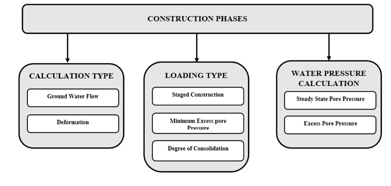
4.3.2. Construction Phases
The FE calculations are divided into several sequential phases corresponding to a loading or construction stage. The types of calculation, loading, and pore-pressure calculation are defined in each construction phase. Fig. (9) shows a flowchart of the construction phases.
4.4. Error Tolerances
4.4.1. Convergence Criteria
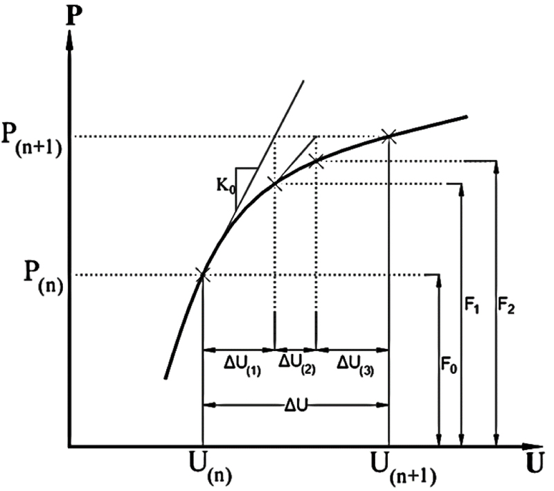
The basic equilibrium equation for the FE analysis is
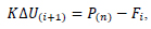 |
(1) |
Where, P is the vector of applied loads, F is the vector of internal forces, ∆U is the vector of nodal displacements, and K is the nonlinear stiffness. For accurate nonlinear analysis, the load P is applied in many load steps n. Eq. (1) is normally solved using several iterations i, the main aim being to determine ∆U. As shown in Fig. (10), as the number of iterations increases, the load imbalance P(n+1)-Fi decreases and the displacement increment also approaches zero U(i) leading to the true solution of the displacement U(i+1) .
4.4.2. Stopping Criteria
Various stopping criteria can be used to decrease the number of unnecessary iterations, such as the following.
• Absolute energy criterion
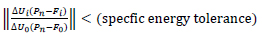 |
(2) |
• Square-root energy criterion
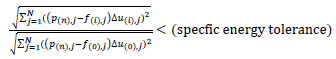 |
(3) |
For a given load step, these criteria correspond to the solution found when the current state's energy imbalance becomes a small fraction of the initial energy imbalance.
• Force criterion: stop when the current force imbalance becomes a small fraction of the total applied force.
• Displacement criterion: stop when the current displacement increment becomes a small fraction of the initial displacement.
In the present case study, the force criterion is used as the stopping criterion. The global error tolerance is 0.01, the maximum number of iterations is 60, and the number of load steps is 1.
CONCLUSION
Recent FE software is inadequate for analyzing vast geotechnical engineering problems. Geotechnical FE analysis is highly dependent on a correct understanding of the soil behavior, parameters, and soil-structure interaction. The flowchart in Fig. (1) describes the main stages of geotechnical FE modeling, along with an illustrative numerical example summarized in Table 1. The primary phase that significantly impacts the behavior and results of the geotechnical FE model is that the 3D geometry plotting model acts as the most realistic geometry used with suitable computing power and time consumed. The deformation and stress at the model boundaries tend to be zero. The Mohr-Coulomb criterion is a suitable constitutive model for any soil type to determine preliminary behavior results in order to increase the accuracy of results; a specific constitutive model could be used as described in Table 5. To ensure the success of the FE model, its results must be checked for their validity, sensitivity, and precision.
APPENDIX
Case Study with Full Details [13]
Initial Purpose
The principal aim is to present 3D numerical analyses based on the FE technique to predict and mitigate the impact of minimum overburden depth for the Nile crossing tunnel. The numerical modeling was developed to simulate soil-tunnel interactions using the commercial 3D FEM program MIDAS/GTSNX powered by TNO-Diana’s solver. The general work sequence of GTS is as follows:
A. Ground and Structural Materials
B. Properties of used mesh element
C. Geometry Modeling
i. Create terrain surfaces from geometric data.
ii. Create a tunnel section.
iii.Extrude to generate 3D modeling.
iv. Make a shared face between solids.
v. Create dividing tool surfaces that represent construction stages.
D. Mesh Generation
The mesh size must be controlled to get a high-quality mesh with fewer meshes; this can be done quickly using the size control. In the [Auto-Solid] Tab, 'Tetra Mesh' and the 'Hybrid Mesh' can be chosen for any geometry.
E. Boundary Condition
In 3D model analysis, constraint displacement is applied in x-direction left/right, y-direction front/back, x,y, and z directions for the bottom part. GTS automatically recognizes the model boundary and sets the boundary condition.
F. Definition of the static loads
For static load, define self-weight, construction loads, surcharge.
G. Analysis condition
Select the analysis type (construction analysis, linear analysis). Then, control analysis and output type in the advance options.
H. Perform Solver
For Post-processing and Result Evaluation: After the analysis is done, the software automatically switches to post-mode (checking results). After the analysis is completed correctly, GTS will organize and provide the post-data result for the design process.
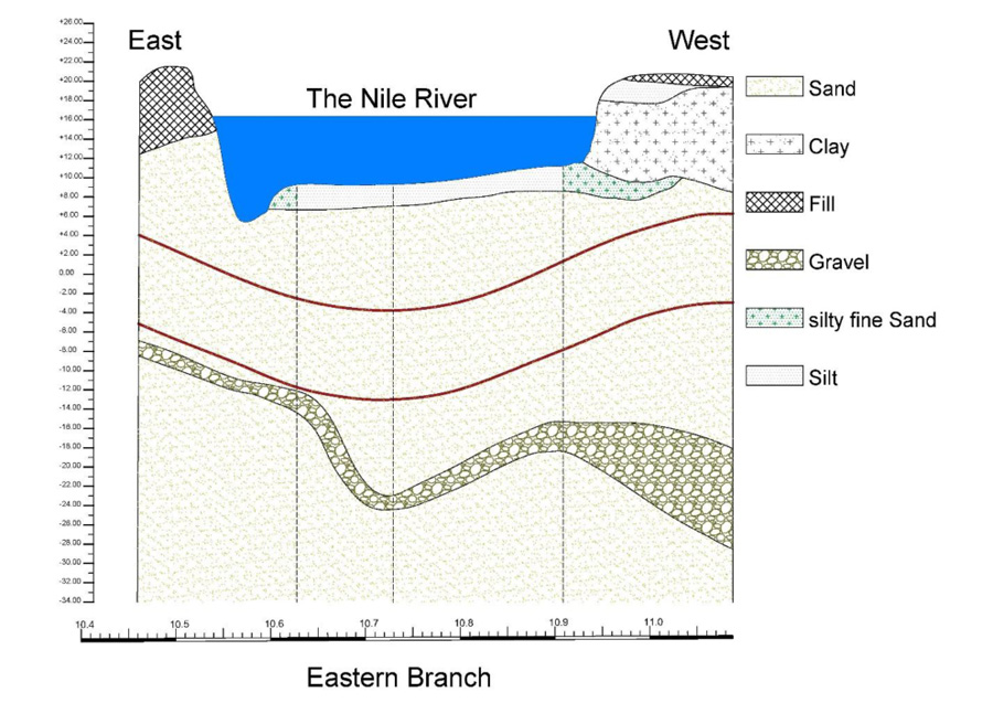
Data Collection
The study was conducted on the most critical section of the Greater Cairo Metro Line 2 tunnel under the Nile River. Fig. (1A) shows the geological section of the case study.
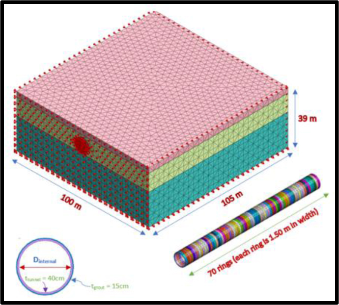
The details of the bored shield tunnel embedded in the soil are as follows: tunnel diameter = 9.15 m,
lining thickness = 0.40m, burial depth (H) = 12 m from the ground surface, segment width = 1.5 m, and grout thickness = 0.15 m.
A local backfilling of the main branch bed is foreseen to ensure a sufficient covering for the shield bored tunnel. Riprap and gravel filters can be modeled as an average weight on the river bed with 60 m width.
Model Establishment
Geometry Plotting
The generation of the geometric model is the foundation of creating a finite element analysis model in GTS.
The dimensions of the overall model in the x, y, and z directions are 100.00×105.00×39.00 m (Fig. 2A). The burial depth (H) is assumed to be 5.50 m from the Nile bed. The water height is 10.00 m over the bed level.
Model Boundary
Midas/GTSNX is capable of constraining the model automatically. The nodal DOF along the vertical sides of the model have been constrained in the X-direction. On the other hand, for the front and back, it is constrained in the Y direction. For bottom nodes, the DOFs of the Z-direction have been constrained with y and x directions.
Model Development
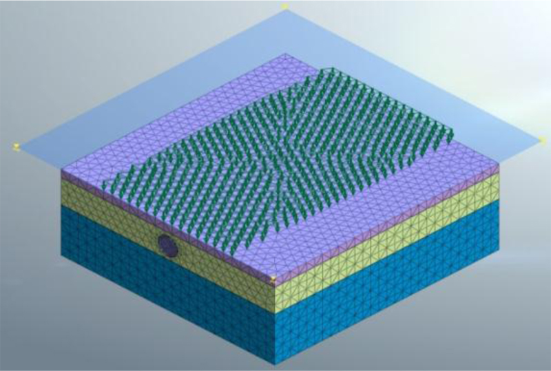
Meshing
Mesh is generated on the previously created geometry model. For a complex model, it is reasonable to use tetrahedron elements or triangular elements produced by the auto-mesh generation function provided by GTS.
Solid elements were chosen for ground, tunnel, and grout. The essential part of mesh generation is the node connection between adjacent elements to form tetrahedron mesh. Solid elements have three translational degrees of freedom in each element node and no rotational degrees of freedom.
Constitutive Model
The soil behavior is simulated using the non-associated Mohr-Columb (MC) criteria, the most widely used method for ground materials due to its simplicity and accuracy (Table 1A).
The structure (shield, tunnel, and grout) 'Elastic' model type that does not consider material nonlinearity is used, as shown below (Table 2A).
Construction Analysis
Active/reactive elements and loads present simulations of the progressive advancement of the TBM. It reflects the change in material properties. It starts from the initial condition of the ground before the commencement of any construction events. The analytical results from the previous stage are accumulated and reanalyzed.
| Material | The Thickness of Layer [m] |
Modulus of Elasticity (E) [kN/m2] |
Poisson’s Ratio (ν) |
Unit Weight (γ) [kN/m3] |
Cohesion (cu) [kN/m2] |
Friction Angle (Φ) [0] |
|---|---|---|---|---|---|---|
| Upper sand | 3.80 | 20000 | 0.30 | 19.00 | 0.00 | 30.00 |
| Middle sand | 12.30 | 75000 | 0.30 | 20.00 | 0.00 | 36.00 |
| Lower sand | 23.00 | 90000 | 0.35 | 20.00 | 0.00 | 40.00 |
| Materials | Modulus of Elasticity (E) [kN/m2] | Poisson's Ratio (ν) | Unit Weight (γ) [kN/m3] |
|---|---|---|---|
| Concrete short term | 2.85×10⁷ | 0.20 | 25.00 |
| Concrete long term | 1.516×10⁷ | 0.20 | 25.00 |
| Shield | 2.00×10⁸ | 0.30 | 75.00 |
| Hard Grout | 50000 | 0.30 | 23.00 |
| Soft Grout | 1000 | 0.30 | 11.00 |
Construction Loads
The main construction loads applied in this study are illustrated in Table 3A and Fig. (3A).
| Pressure Type |
Value [kN/m2] |
|---|---|
| Face pressure | 200 |
| Grout pressure | 300 |
| Jacking pressure | 4600 |
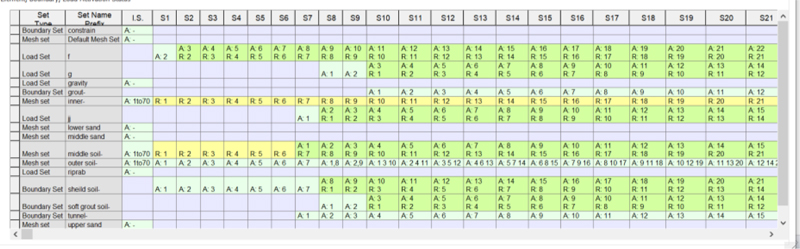
Construction Stages
A stage-by-stage analysis is employed to simulate the progress of the TBM and the tunnel construction process. The tunnel is divided into 70 rings constructed in 79 stages. The length of the shield is 10.5 m simulated in the model as a ring with a width of 1.5 m. The face pressure is normal on the excavated soil at the shield face. The soft grout is pumped from the tail of the shield by grouting pressure towards the soil to prevent it from collapsing. The grout results in a compressive force on the segments. The jacking force is rested on the tunnel segment to push the machine to advance.
It is assumed that the grout hardened after two constructed rings, and the grout pressure was simulated considering the soft grout strata. These stages are illustrated in Fig. (4A) and as follows:
- Initial Stage (IS): This stage simulated the initial state of stresses in the terrain before tunneling construction.
- Stage 1 (S1): In this stage, the excavation of the first ring is simulated, and the shield replaces it. The face pressure is released from the start position to be applied to the next ring.
- Stage 2 to 6 (S2:S6): in this stage, the same simulation explained in stage 1 is repeated to excavate the 2nd ring to the sixth ring and replace them with the shield.
- Stage 7 (S7): In this stage, excavation of the seventh ring is simulated and replaced by the shield. With the progression of a machine, the shield's tail exists in the first excavated ring. In the meantime, the first tunnel segments are constructed, and jacking is released.
- Stage 8 (S8): In this stage, excavation of the eighth ring is simulated, and the shield replaces it. With the machine's progression, the shield's tail is released from its position to the second excavated ring, and the shield is present inside the soil with a total length of 10.5 m.
- Stage 9 (S9): In this stage, excavation of the ninth ring is simulated and replaced by the shield. With the progression of the machine, the tail of the shield is released from its position to the third excavated ring.
- Stage 10 (S10): The tenth ring is simulated and replaced by the shield in this stage. With the progression of the machine, the tail of the shield is released from its position to the fourth excavation ring.
- Stage n (Sn): In this stage, excavation of the nth ring is simulated and replaced by the shield. With the progression of the machine, the tail of the shield is released from its position to the next excavated ring. In the meantime, the tunnel segments are constructed, and the jacking is released from its position to be applied on the next. The grout pressure is acted on the perimeter of the segments toward the soil and released before the previous segments, and the hard grout is applied to them. This stage is repeated until all segments are constructed.
Backfilling
A local backfilling of the main branch bed is foreseen to ensure a sufficient covering for the shield bored tunnel. Riprap and gravel filters can be modeled as an average weight on the river bed with 60 m width. For the short term, the weight of backfilling is 28.00kN/m2. For the long-term and exceptional case, the weight of backfilling is 12.00kN/m2. Fig. (5A) illustrates the backfilling load.
Model Results
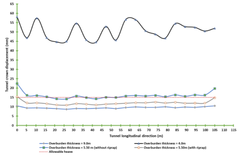
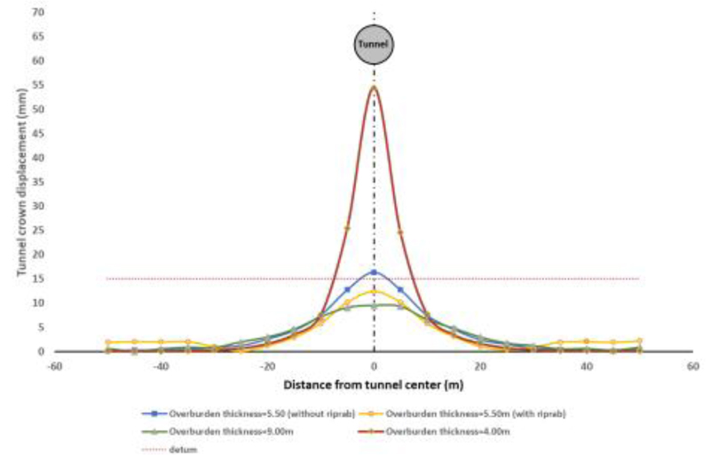
The vertical displacement at the crown of the tunnel during different stages of the tunnel's construction and in-service case were studied. The 3D analysis results (Fig. 6A) showed that the crown vertical displacement value was 18.8 mm. If the cover thickness is less than the theoretical calculation, this is called a critical section. The cover begins approximately one diameter ahead of the tunnel face; the crown vertical displacement value is about 11.1 mm, decreasing by a ratio of 40%. The critical section has a 5.50 m cover. Two models with/without riprap conduct analyses; in the model with riprap, the maximum heave equals 11.6 mm, but for the model without riprap, the heave is equal to 13.9 mm.
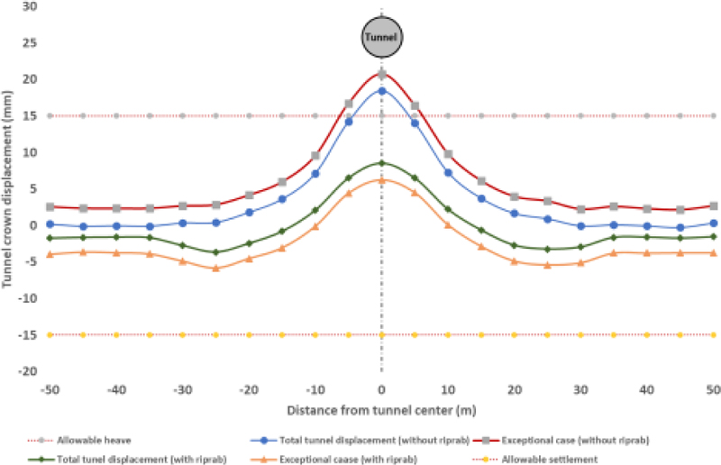
For the long and short-term combination, the total crown vertical heave is 15.99 mm for the model without riprap and 9.99 mm for the model with riprap by decreasing the ratio by approximately 40% (Fig. 6A).

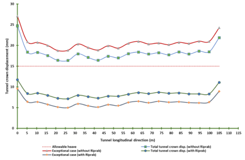
For the exceptional case, the total crown vertical heave is 18.26 mm for the model without riprap and 8.38 mm for the model with riprap by decreasing the ratio by approximately 54% (Fig. 7A).
CONCLUSION
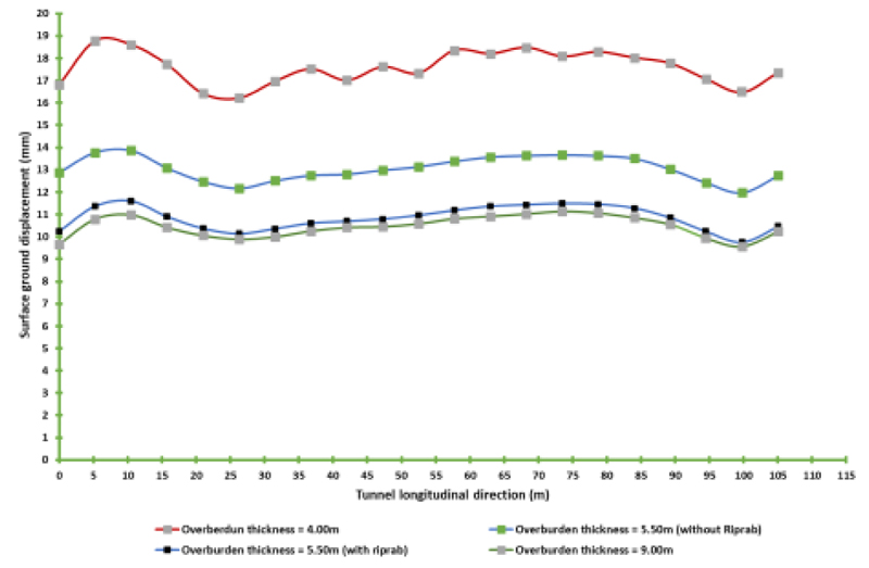
The surface displacement should be less than the design value (±15 mm). If the cover begins approximately one diameter ahead of the tunnel face, the crown vertical displacement value is about 10.50 mm.
For model with cover thickness 5.5m with/without riprap, the following is noticed:
- The surface heave decreases by 21–31% during construction, as shown in Figs. (7A and 9A).
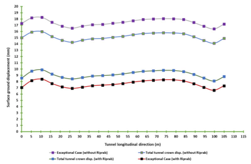
- The surface heave decreases by 59 - 65% for short-term and long-term combinations, as shown in Figs. (8A and 11A).
- For the models during the exceptional case, the surface heave decreases by 63 - 73%, as shown in Figs. (8A and 10A).
CONSENT FOR PUBLICATION
Not applicable.
FUNDING
None.
CONFLICT OF INTEREST
The authors declare no conflict of interest, financial or otherwise.
ACKNOWLEDGEMENTS
Declared none.