All published articles of this journal are available on ScienceDirect.

Behavior of Fibrous Reinforced Concrete Splices
Abstract
Background:
The tangent of the relationship between bond stress and displacement (slip) is called the modulus of displacement and gives the basis for the theory. This theory is used to determine the stress distribution along the spliced reinforcement bars.
Objective:
This research presents a modification on the theory of the modulus of displacement to determine the stress distribution along the spliced reinforcement bond for fibrous reinforced concrete.
Methods:
1- General differential equations are derived for concrete stress, stress in reinforcement bars and bond stress between reinforcement bars and surrounding concrete.
2-The general solutions of these D.E. are determined and Excel data sheets are prepared to apply these solutions and determine the concrete, steel and bond stresses.
Results:
Excel data sheets are prepared to determine the concrete, steel and bond stresses. The stresses are determined along the bar splice length considering the effect of steel fiber content.
Conclusion:
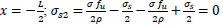
The maximum concrete stress is obtained at center x=0 and minimum at
 . Maximum bond stress obtained at
and minimum at the center. The maximum steel stress at
. Maximum bond stress obtained at
and minimum at the center. The maximum steel stress at
 and minimum at
 . The value of (σcmax) increased linearly with increasing of (ρ). The concrete stress increased nonlinearly with (ρ%) and linearly with ( fy) and (fc’). Also increasing of (k) and bar diameter have small effects. The value of bond stress decreased linearly with (Qf) and (ρ%).
1. INTRODUCTION
Modulus of displacement theory is used to determine the stress distribution along the spliced reinforcement bars. The tangent of the relationship between bond stress and displacement (slip) is called the modulus of displacement and gives the basis for the theory. Fig. (1) shows the relation between bond stress and displacement (slip).
Losberg investigated the bond properties of long concrete specimens with pulled, axially embedded reinforcement bars [1]. He used the modulus of displacement theory for the calculation of the stresses and the crack widths. Also, he extended the investigations to the curtailment of reinforcement in accordance with the moment diagram, and the influence of cracks was also studied.
Feldman and Bartlett showed that bond stress magnitude varies along the length of plain reinforcing bars in pullout specimens by using analytical methods and experimental tests [2]. They established analytical relationships between bond stress and slip at the unloaded end of the bar and along the length of the bar. The analytical relationship showed that the bond stress is a function of bar slip, slip is a function of bar force, and bar force is a function of bond stress. Also, they concluded that the maximum load occurs just before slip occurs at the unloaded end of the bar, and the location of the peak bond stress shifts from the loaded end towards the unloaded end of the specimen with increasing applied load.
Thompson et al. studied the anchorage behavior of headed reinforcement in lap splices by experimental tests [3]. They concluded that the stress is transferred between opposing bars in non-contact lap splices through struts acting at an angle to the direction of the bar. Anchorage length in non-contact lap splices could be determined by drawing the struts between opposing bars propagate at an angle of 55° with respect to the bar axis.
Coogler et al. tested two commercially available offset mechanical splice systems in direct tension with the splice both restrained and unrestrained from rotation [4]. They concluded that pullout failure was the most common failure mode observed. This mode of failure results in a decrease in apparent ultimate stress for the system because of the inability to develop the full strength of the cross-section. A 345 MPa stress range for fatigue testing results in fatigue-induced reinforcing bar rupture at a very low number of cycles. A more reasonable stress range of 138 MPa is suggested for assessing the performance of this type of splice. Also, for all in-place testing, concrete was unable to properly confine the offset splice near ultimate load levels.
Feldman and Bartlett concluded that there is a complicated interaction between flexural and shear behavior, band stress, and cracking two full-scale T-beams, 4.2m long with a/d=7.5 were tested in four-point loading [5]. Both were reinforced with plain hollow steel bars that had roughened surfaces to simulate bars found in historic structures. The flexural reinforcement ratios were 0.33% for the HSS bar and 0.98% for plane bars. Arch action initiated in the beam reinforced with plane bars due to loss of bond in the constant shear region near midspan when the applied load reached 60% of its maximum value. The beam reinforced with the HSS bars had lesser bond demand, and arch action due to bond loss did not initiate in the beam until the maximum load was achieved. Also, when shear is carried by beam action, bond demand is greatest within the elastic-uncracked region adjacent to the first flexural crack.
Yang and Ashour developed a mechanical analysis based on an upper-bound theorem to predict the optimum failure surface and concrete breakout capacity of single anchors under tensile loads [6]. The predicted results obtained from ACI 318-05 are compared with the experimental test results. They concluded that the shape of the failure surface predicted by the mechanism analysis is significantly influenced by the ratio of effective tensile and compressive strengths of concrete. The concrete breakout capacity of anchors predicted from mechanism analysis responds sensitively to the variation of the ratio between effective tensile and compressive strengths of concrete. Conservation of ACI 318-05 sharply increases in specimens having concrete strength above 50 MPa, whereas the mechanism analysis shows good agreement with tests results, regardless of concrete strength.
Sezen and Setzler showed that the contribution of bar slip deformations to total member lateral displacement could be significant [7]. In addition to flexural deformations, bar slip deformations should be considered in the modeling and analysis of reinforced concrete members. They present a method for computing slip for bars stressed, its unloaded end, and hooked bars. The proposed model is compared with five models found in the literature and three independent sets of experimental data. Also, the proposed model is used to calculate the lateral load-slip displacement relations for seven columns from two different studies, and the computed relations compare well with the measured test results.
Howell and Higgins studied the bond performance of square and round deformed reinforcing bars [8]. They concluded that the application of the simplified ACI development length equations to characterize the reinforcing bar stress provided a reasonable lower bound for both square and round bars across all test types. Also, the ACI approach was conservative for partial reinforcing bar embedment of round and square results and indicated that linear interpolation of available reinforcing bar stress for embedment lengths less than the computed development length also appears reasonable for the square reinforcing bar. Computation of development length using the ACI formula with an equivalent round diameter for square reinforcing bar results in lengths (13%) larger than when the side dimension is used. This is conservative and available for large square reinforcing bar sizes and alternative test configurations.
Eligehausen et al. proposed a model to predict the average failure load of anchorage using adhesive banded anchors based on numerical and experimental investigations [9]. The model is similarly cast in place, and post-installed mechanical anchors are incorporated in ACI 318-05, but with the following modifications:
(1) The basic strength of a single adhesive anchor predicts the pullout capacity and not the concrete breakout capacity.
(2) The critical spacing and critical edge distance of adhesive anchorages depend on the anchor diameter and the bond strength and not on the anchor embedment depth.
(3) The proposed model results agree very well with the results of (415) group tests contained in a worldwide database.
This research presents a modification on the theory of the modulus of displacement that has been presented by Tepfors [10] to determine the stress distribution along the spliced reinforcement bond for fibrous reinforced concrete.
2. MATERIALS AND METHODS
2.1. Theoretical Analysis
2.1.1. Basic Equations
- 1- The splice area is located in the region of the constant moment and has no shear.
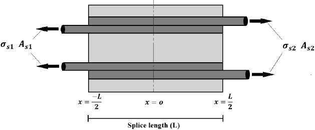
- 2- The stress in the reinforcement at both ends of the splice is equal.
- 3- Moment cracks in the concrete are located at the ends of the splice, and the stress in the reinforcement is (σs). Fig. (2) shows the tension reinforcement splice.
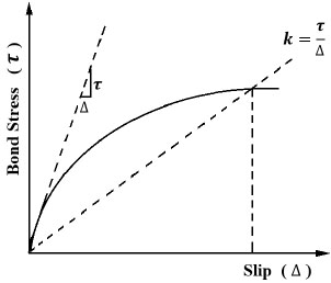
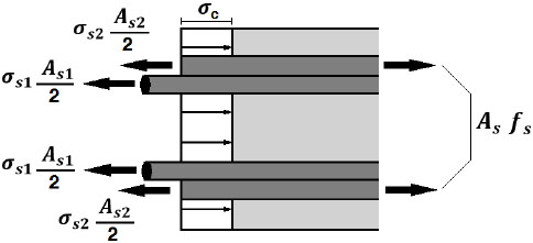
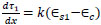
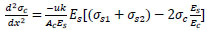
From Fig. (1); the bond stress between reinforcement and concrete:
 |
(1) |
Where τ= bond stress. (MPa) N/mm2
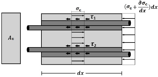
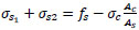
The connection between bond stress (τ) and normal stress of concrete (
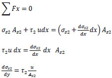
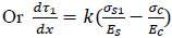
The horizontal equilibrium of splice bar at
 gives the following equations:
 |
(2) |
Also by the same way:
 |
(3) |
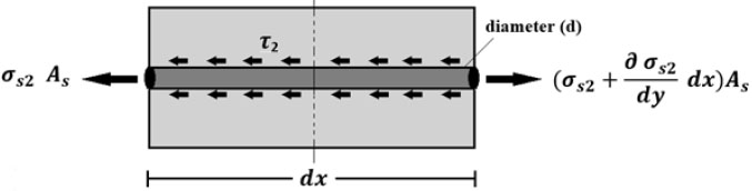
Where: d = diameter of the bar (mm).
τ1 = band stress at x=-
 (MPa)
(MPa)
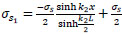
σs1 = tension steel stress at
(MPa)
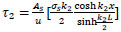
τ2 = band stress at x=
(MPa)
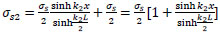
σs2 = tension stress at x=-
(mpa)
Concrete stress is determined from the horizontal equilibrium of the concrete steel connection shown in Fig. (4);
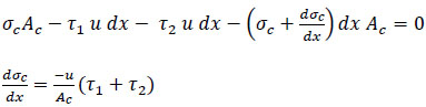 |
(4) |
Where
The equilibrium condition for the splice is shown in Fig. (5)
 |
(5) |
Where:
From Eq.(1); derivate on both sides :
 |
(6) |
The strain is the difference in displacement between the two materials, concrete, and steel.
 |
(7) |
The change in shear stress for element length (
 |
(8) |
Or
 |
(9) |
And
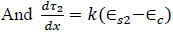 |
(10) |
Or
 |
(11) |
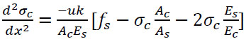
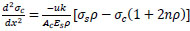
Take the derivative of both sides of Eq. (4);
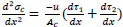 |
(12) |
Substitute Eq. (9 and 11) into Eq. (12) to get;
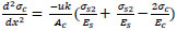 |
(13) |
 |
(14) |
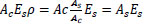
From Eq. (5);
 |
(15) |
the bar diameter is taken the same at both side of the splice, thus:
 |
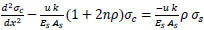
Subacute Eq. (15) into Eq. (14);
 |
(16) |
taking 
and n = modular ratio =

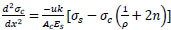 |
(17) |
 |
(18) |
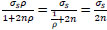
but
re-arrange Eq. (18) to get:
 |
(19) |
Let
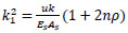
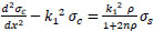 |
(20) |
The general solution of Eq. (20) is:
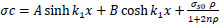 |
(21) |
The constants A and B are determined by application of the boundary conditions:
at
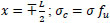 for fibrous concrete
The tensile strength of plain concrete with steel fiber can be calculated from the following equations (11, 12).
σfu =0.82τF
where: τ = Interfacial bond strength between steel fiber and concrete matrix.

Q f = volume fraction of steel fiber (%).
d f = Bond factor depends on the type of steel fiber.
L f = Length of steel fiber (mm).
D f = Diameter of steel fiber (mm).
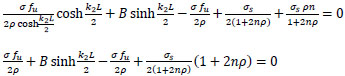
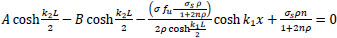
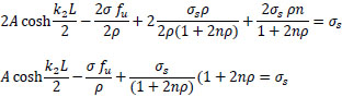
These give the constants as:
 |
(22) |
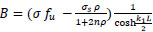 |
(23) |
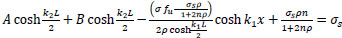
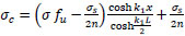
The final form of the concrete normal stress is:
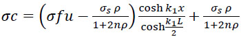 |
(24) |
for concrete without steel fiber: σ fu=0;
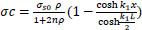 |
(25) |
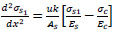
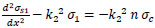
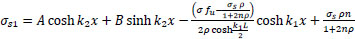
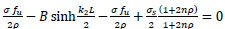
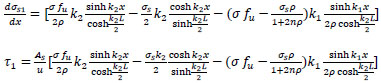
The normal stress (σs1) is determined by derivation of Eq. (3) and combined with Eq. (9) to get:
 |
(26) |
 |
(27) |
rearrangement of Eq. (27);
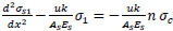 |
(28) |
Let

 |
(29) |
The homogeneous solution of Eq. (29) is:
 |
(30) |
because of σc is also a function of (x), thus the particular solution is taken as the following:
 |
(31) |
Substitute σs1ρ & its 2nd derivative into eq. (29) to find the constants C, D, & E.
 |
(32) |
substitute Eqs. (31 and 32) into Eq. (29);
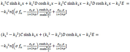 |
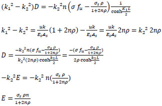 |
finally:
or
 |
(33) |
for concrete without steel fiber; σ fu=0;
 |
(34) |
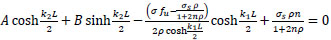
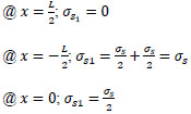
Applying B.C.:
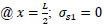
and x=-
; σs1 = σs
 |
(35) |
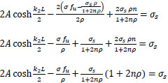
 |
(36) |
adding the above two equations:
 |
 |
(37) |
substitute in Eq. (35);
 |
 |
(38) |
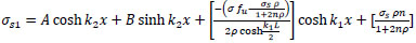
Finally:
 |
or
 |
(39) |
Check: @

 |
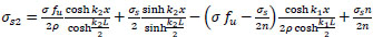
By the same way. The derivation of Eq. (2) is combined with Eq. (11) to get;
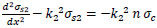 |
(40) |
By the same previous procedures, the general solution is:
 |
(41) |
The B.C. are:
@x=-
; σs2 = σs
@x=-
;σs2 = 0
 |
(42) |
 |
(43) |
adding the above two equations:
 |
 |
(44) |
sub. in Eq. (42);
 |
 |
 |
(45) |
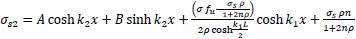
Finally:
 |
(46) |
Check: @

@
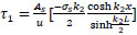
The bond stresses ( & x=-
are determined from Eqs. (2 & 3):
 |
(47) |
 |
(48) |
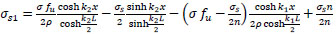
from Eq. (39);
 |
(49) |
from Eq. (46);
 |
(50) |
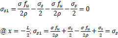
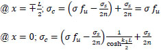
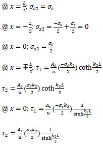
For the special case:
when ρ = ∞ ; at x = ∓
; concrete cracks and
 |
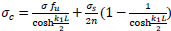
from Eq. (24);
 |
(51) |
 |
 |
for concrete without fiber,
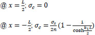 |
from Eq. (39);
 |
 |
(52) |
 |
and from Eq. (49);
 |
(53) |
 |
 |
(54) |
from Eq. (50);
 |
(55) |
 |
3. RESULTS AND DISCUSSION
Effect of steel fiber content is considered on the bond stress between steel bars and surrounding fibrous concrete and concrete stress at the lap splice, taking into account the following variables:
- 1- Steel fiber content
( Q f % ) . - 2- Value of modulus of displacement
k N / m m 3 - 3- Reinforcement index
( ρ % ) . - 4- Bar diameter
( d b ) m m . - 5- Steel bar yield strength
( f y ) N / m m 2 - 6- Compressive strength of concrete
f c ' N / m m 2
Excel data sheets are prepared to apply equations of concrete stress (σc), steel stress (σs), and bond stress
| K(N/mm^3) = | 50 | 100 | 150 | 50 | 100 | 150 | 50 | 100 | 150 | 50 | 100 | 150 |
| L (mm) = | 500 | 500 | 500 | 500 | 500 | 500 | 500 | 500 | 500 | 500 | 500 | 500 |
| Fy(N/mm^2)= | 420 | 420 | 420 | 420 | 420 | 420 | 420 | 420 | 420 | 420 | 420 | 420 |
| Rho % = | 1 | 1 | 1 | 1 | 1 | 1 | 1 | 1 | 1 | 1 | 1 | 1 |
| Qf (fiber) %= | 0 | 0 | 0 | 0.5 | 0.5 | 0.5 | 1 | 1 | 1 | 2 | 2 | 2 |
| L/D Fiber = | 100 | 100 | 100 | 100 | 100 | 100 | 100 | 100 | 100 | 100 | 100 | 100 |
| df fiber = | 1 | 1 | 1 | 1 | 1 | 1 | 1 | 1 | 1 | 1 | 1 | 1 |
| fc'(N/mm^2)= | 28 | 28 | 28 | 28 | 28 | 28 | 28 | 28 | 28 | 28 | 28 | 28 |
| Es(N/mm^2)= | 200000 | 200000 | 200000 | 200000 | 200000 | 200000 | 200000 | 200000 | 200000 | 200000 | 200000 | 200000 |
| bar diameter= | 10 | 10 | 10 | 10 | 10 | 10 | 10 | 10 | 10 | 10 | 10 | 10 |
| F= | 0 | 0 | 0 | 0.5 | 0.5 | 0.5 | 1 | 1 | 1 | 2 | 2 | 2 |
| Sigma fu= | 0 | 0 | 0 | 1.7015 | 1.7015 | 1.7015 | 3.403 | 3.403 | 3.403 | 6.806 | 6.806 | 6.806 |
| u= | 31.4159 | 31.4159 | 31.4159 | 31.4159 | 31.4159 | 31.4159 | 31.4159 | 31.4159 | 31.4159 | 31.4159 | 31.4159 | 31.4159 |
| As= | 78.53975 | 78.53975 | 78.53975 | 78.53975 | 78.53975 | 78.53975 | 78.53975 | 78.53975 | 78.53975 | 78.53975 | 78.53975 | 78.53975 |
| Ec= | 25034.099 | 25034.099 | 25034.099 | 25034.099 | 25034.099 | 25034.099 | 25034.1 | 25034.1 | 25034.099 | 25034.099 | 25034.1 | 25034.099 |
| n= | 7.9891032 | 7.9891032 | 7.9891032 | 7.9891032 | 7.9891032 | 7.9891032 | 7.989103 | 7.989103 | 7.9891032 | 7.9891032 | 7.989103 | 7.9891032 |
| K2^2= | 0.00010 | 0.00020 | 0.00030 | 0.00010 | 0.00020 | 0.00030 | 0.00010 | 0.00020 | 0.00030 | 0.00010 | 0.00020 | 0.00030 |
| K1^2= | 0.000116 | 0.000232 | 0.0003479 | 0.000116 | 0.000232 | 0.0003479 | 0.000116 | 0.000232 | 0.0003479 | 0.000116 | 0.000232 | 0.0003479 |
| K1*L/2= | 2.6923295 | 3.8075288 | 4.6632514 | 2.6923295 | 3.8075288 | 4.6632514 | 2.692329 | 3.807529 | 4.6632514 | 2.6923295 | 3.807529 | 4.6632514 |
| K2*L/2= | 2.5 | 3.5355339 | 4.330127 | 2.5 | 3.5355339 | 4.330127 | 2.5 | 3.535534 | 4.330127 | 2.5 | 3.535534 | 4.330127 |
| Fy*Rho/(1+2nRho)= | 3.62137 | 3.62137 | 3.62137 | 3.62137 | 3.62137 | 3.62137 | 3.62137 | 3.62137 | 3.62137 | 3.62137 | 3.62137 | 3.62137 |
| Sfu - above = | -3.62137 | -3.62137 | -3.62137 | -1.91987 | -1.91987 | -1.91987 | -0.21837 | -0.21837 | -0.21837 | 3.18463 | 3.18463 | 3.18463 |
| K2= | 0.01 | 0.0141421 | 0.0173205 | 0.01 | 0.0141421 | 0.0173205 | 0.01 | 0.014142 | 0.0173205 | 0.01 | 0.014142 | 0.0173205 |
| K1= | 0.0107693 | 0.0152301 | 0.018653 | 0.0107693 | 0.0152301 | 0.018653 | 0.010769 | 0.01523 | 0.018653 | 0.0107693 | 0.01523 | 0.018653 |
| Cosh(K1L/2)= | 7.4168779 | 22.530603 | 52.994771 | 7.4168779 | 22.530603 | 52.994771 | 7.416878 | 22.5306 | 52.994771 | 7.4168779 | 22.5306 | 52.994771 |
| Cosh(K2L/2)= | 6.1322895 | 17.171237 | 37.98355 | 6.1322895 | 17.171237 | 37.98355 | 6.132289 | 17.17124 | 37.98355 | 6.1322895 | 17.17124 | 37.98355 |
| - | - | - | - | - | - | - | - | - | - | - | - | - |
| X | Sc(Concrete) | Sc(Concrete) | Sc(Concrete) | Sc(Concrete) | Sc(Concrete) | Sc(Concrete) | Sc(Concrete) | Sc(Concrete) | Sc(Concrete) | Sc(Concrete) | Sc(Concrete) | Sc(Concrete) |
| -250 | 0 | 0 | 0 | 1.7015 | 1.7015 | 1.7015 | 3.403 | 3.403 | 3.403 | 6.806 | 6.806 | 6.806 |
| -200 | 1.4891048 | 1.9273371 | 2.1956344 | 2.4909492 | 2.7232781 | 2.865516 | 3.492794 | 3.519219 | 3.5353976 | 5.4964824 | 5.111101 | 4.8751608 |
| -150 | 2.3448858 | 2.823921 | 3.0585701 | 2.9446417 | 3.1986023 | 3.3230015 | 3.544398 | 3.573284 | 3.587433 | 4.7439093 | 4.322646 | 4.1162959 |
| -100 | 2.8215263 | 3.2352882 | 3.3954314 | 3.1973327 | 3.4166887 | 3.5015886 | 3.573139 | 3.598089 | 3.6077458 | 4.3247519 | 3.96089 | 3.8200602 |
| -50 | 3.0605979 | 3.4117395 | 3.5210979 | 3.3240766 | 3.5102344 | 3.5682107 | 3.587555 | 3.608729 | 3.6153236 | 4.1145126 | 3.805719 | 3.7095492 |
| 0 | 3.1331093 | 3.4606389 | 3.5530355 | 3.3625185 | 3.5361584 | 3.5851425 | 3.591928 | 3.611678 | 3.6172494 | 4.0507461 | 3.762717 | 3.6814633 |
| 50 | 3.0605979 | 3.4117395 | 3.5210979 | 3.3240766 | 3.5102344 | 3.5682107 | 3.587555 | 3.608729 | 3.6153236 | 4.1145126 | 3.805719 | 3.7095492 |
| 100 | 2.8215263 | 3.2352882 | 3.3954314 | 3.1973327 | 3.4166887 | 3.5015886 | 3.573139 | 3.598089 | 3.6077458 | 4.3247519 | 3.96089 | 3.8200602 |
| 150 | 2.3448858 | 2.823921 | 3.0585701 | 2.9446417 | 3.1986023 | 3.3230015 | 3.544398 | 3.573284 | 3.587433 | 4.7439093 | 4.322646 | 4.1162959 |
| 200 | 1.4891048 | 1.9273371 | 2.1956344 | 2.4909492 | 2.7232781 | 2.865516 | 3.492794 | 3.519219 | 3.5353976 | 5.4964824 | 5.111101 | 4.8751608 |
| 250 | 0 | 0 | 0 | 1.7015 | 1.7015 | 1.7015 | 3.403 | 3.403 | 3.403 | 6.806 | 6.806 | 6.806 |
| K(N/mm^3) = | 50 | 100 | 150 | 50 | 100 | 150 | 50 | 100 | 150 | 50 | 100 | 150 |
| L (mm) = | 500 | 500 | 500 | 500 | 500 | 500 | 500 | 500 | 500 | 500 | 500 | 500 |
| Fy(N/mm^2)= | 420 | 420 | 420 | 420 | 420 | 420 | 420 | 420 | 420 | 420 | 420 | 420 |
| Rho % = | 1 | 1 | 1 | 1 | 1 | 1 | 1 | 1 | 1 | 1 | 1 | 1 |
| Qf (fiber) %= | 0 | 0 | 0 | 0.5 | 0.5 | 0.5 | 1 | 1 | 1 | 2 | 2 | 2 |
| L/D Fiber = | 100 | 100 | 100 | 100 | 100 | 100 | 100 | 100 | 100 | 100 | 100 | 100 |
| df fiber = | 1 | 1 | 1 | 1 | 1 | 1 | 1 | 1 | 1 | 1 | 1 | 1 |
| fc'(N/mm^2)= | 28 | 28 | 28 | 28 | 28 | 28 | 28 | 28 | 28 | 28 | 28 | 28 |
| Es(N/mm^2)= | 200000 | 200000 | 200000 | 200000 | 200000 | 200000 | 200000 | 200000 | 200000 | 200000 | 200000 | 200000 |
| bar diameter= | 10 | 10 | 10 | 10 | 10 | 10 | 10 | 10 | 10 | 10 | 10 | 10 |
| F= | 0 | 0 | 0 | 0.5 | 0.5 | 0.5 | 1 | 1 | 1 | 2 | 2 | 2 |
| Sigma fu= | 0 | 0 | 0 | 1.7015 | 1.7015 | 1.7015 | 3.403 | 3.403 | 3.403 | 6.806 | 6.806 | 6.806 |
| u= | 31.4159 | 31.4159 | 31.4159 | 31.4159 | 31.4159 | 31.4159 | 31.4159 | 31.4159 | 31.4159 | 31.4159 | 31.4159 | 31.4159 |
| As= | 78.53975 | 78.53975 | 78.53975 | 78.53975 | 78.53975 | 78.53975 | 78.53975 | 78.53975 | 78.53975 | 78.53975 | 78.53975 | 78.53975 |
| As/u= | 2.5 | 2.5 | 2.5 | 2.5 | 2.5 | 2.5 | 2.5 | 2.5 | 2.5 | 2.5 | 2.5 | 2.5 |
| Ec= | 25034.09891 | 25034.099 | 25034.099 | 25034.099 | 25034.099 | 25034.099 | 25034.1 | 25034.1 | 25034.099 | 25034.099 | 25034.1 | 25034.099 |
| n= | 7.989103213 | 7.9891032 | 7.9891032 | 7.9891032 | 7.9891032 | 7.9891032 | 7.989103 | 7.989103 | 7.9891032 | 7.9891032 | 7.989103 | 7.9891032 |
| K2^2= | 0.00010 | 0.00020 | 0.00030 | 0.00010 | 0.00020 | 0.00030 | 0.00010 | 0.00020 | 0.00030 | 0.00010 | 0.00020 | 0.00030 |
| K1^2= | 0.000115978 | 0.000232 | 0.0003479 | 0.000116 | 0.000232 | 0.0003479 | 0.000116 | 0.000232 | 0.0003479 | 0.000116 | 0.000232 | 0.0003479 |
| K1*L/2= | 2.692329456 | 3.8075288 | 4.6632514 | 2.6923295 | 3.8075288 | 4.6632514 | 2.692329 | 3.807529 | 4.6632514 | 2.6923295 | 3.807529 | 4.6632514 |
| K2*L/2= | 2.5 | 3.5355339 | 4.330127 | 2.5 | 3.5355339 | 4.330127 | 2.5 | 3.535534 | 4.330127 | 2.5 | 3.535534 | 4.330127 |
| Fy*Rho/(1+2nRho)= | 3.621370022 | 3.62137 | 3.62137 | 3.62137 | 3.62137 | 3.62137 | 3.62137 | 3.62137 | 3.62137 | 3.62137 | 3.62137 | 3.62137 |
| Sfu - above = | -3.62137002 | -3.62137 | -3.62137 | -1.91987 | -1.91987 | -1.91987 | -0.21837 | -0.21837 | -0.21837 | 3.18463 | 3.18463 | 3.18463 |
| K2= | 0.01 | 0.0141421 | 0.0173205 | 0.01 | 0.0141421 | 0.0173205 | 0.01 | 0.014142 | 0.0173205 | 0.01 | 0.014142 | 0.0173205 |
| K1= | 0.010769318 | 0.0152301 | 0.018653 | 0.0107693 | 0.0152301 | 0.018653 | 0.010769 | 0.01523 | 0.018653 | 0.0107693 | 0.01523 | 0.018653 |
| Cosh(K1L/2)= | 7.416877858 | 22.530603 | 52.994771 | 7.4168779 | 22.530603 | 52.994771 | 7.416878 | 22.5306 | 52.994771 | 7.4168779 | 22.5306 | 52.994771 |
| Cosh(K2L/2)= | 6.13228948 | 17.171237 | 37.98355 | 6.1322895 | 17.171237 | 37.98355 | 6.132289 | 17.17124 | 37.98355 | 6.1322895 | 17.17124 | 37.98355 |
| Sinh(K1L/2)= | 7.34915486 | 22.5084 | 52.985336 | 7.3491549 | 22.5084 | 52.985336 | 7.349155 | 22.5084 | 52.985336 | 7.3491549 | 22.5084 | 52.985336 |
| Sinh(K2L/2)= | 6.050204481 | 17.142093 | 37.970384 | 6.0502045 | 17.142093 | 37.970384 | 6.050204 | 17.14209 | 37.970384 | 6.0502045 | 17.14209 | 37.970384 |
| - | - | - | - | - | - | - | - | - | - | - | - | - |
| X | Tau stress | Tau stress | Tau stress | Tau stress | Tau stress | Tau stress | Tau stress | Tau stress | Tau stress | Tau stress | Tau stress | Tau stress |
| -250 | 10.15167604 | 14.324685 | 17.538596 | 9.9804964 | 14.091373 | 17.25462 | 9.809317 | 13.85806 | 16.970644 | 9.4669576 | 13.39144 | 16.402691 |
| -200 | 6.058717725 | 6.8872504 | 7.1496826 | 6.0038161 | 6.8554463 | 7.1372815 | 5.948914 | 6.823642 | 7.1248804 | 5.8391111 | 6.760034 | 7.1000781 |
| -150 | 3.628961482 | 3.3195417 | 2.9205115 | 3.6214913 | 3.3410165 | 2.9565485 | 3.614021 | 3.362491 | 2.9925856 | 3.5990808 | 3.405441 | 3.0646596 |
| -100 | 2.19181798 | 1.6117052 | 1.2001241 | 2.1987152 | 1.6366736 | 1.2297106 | 2.205612 | 1.661642 | 1.2592971 | 2.219407 | 1.711579 | 1.3184701 |
| -50 | 1.349760541 | 0.8021895 | 0.5061435 | 1.3560495 | 0.81626 | 0.5206444 | 1.362339 | 0.830331 | 0.5351453 | 1.3749166 | 0.858472 | 0.5641471 |
| 0 | 0.867739267 | 0.4331222 | 0.2394831 | 0.8677393 | 0.4331222 | 0.2394831 | 0.867739 | 0.433122 | 0.2394831 | 0.8677393 | 0.433122 | 0.2394831 |
| 50 | 0.607210115 | 0.2897912 | 0.1639454 | 0.6009211 | 0.2757206 | 0.1494445 | 0.594632 | 0.26165 | 0.1349436 | 0.5820541 | 0.233509 | 0.1059417 |
| 100 | 0.486165337 | 0.2751341 | 0.1958602 | 0.4792681 | 0.2501657 | 0.1662737 | 0.472371 | 0.225197 | 0.1366872 | 0.4585763 | 0.17526 | 0.0775142 |
| 150 | 0.453594908 | 0.3455462 | 0.3154513 | 0.4610651 | 0.3240713 | 0.2794143 | 0.468535 | 0.302596 | 0.2433772 | 0.4834756 | 0.259647 | 0.1713032 |
| 200 | 0.470492136 | 0.4662699 | 0.5087599 | 0.5253938 | 0.498074 | 0.521161 | 0.580295 | 0.529878 | 0.5335621 | 0.6900987 | 0.593486 | 0.5583643 |
| 250 | 0.490780712 | 0.5498024 | 0.6542437 | 0.6619603 | 0.7831149 | 0.9382198 | 0.83314 | 1.016427 | 1.2221959 | 1.1754991 | 1.483052 | 1.7901481 |
| K(N/mm^3) = | 50 | 100 | 150 | 50 | 100 | 150 | 50 | 100 | 150 | 50 | 100 | 150 |
| L (mm) = | 500 | 500 | 500 | 500 | 500 | 500 | 500 | 500 | 500 | 500 | 500 | 500 |
| Fy(N/mm^2)= | 420 | 420 | 420 | 420 | 420 | 420 | 420 | 420 | 420 | 420 | 420 | 420 |
| Rho % = | 1 | 1 | 1 | 1 | 1 | 1 | 1 | 1 | 1 | 1 | 1 | 1 |
| Qf (fiber) %= | 0 | 0 | 0 | 0.5 | 0.5 | 0.5 | 1 | 1 | 1 | 2 | 2 | 2 |
| L/D Fiber = | 100 | 100 | 100 | 100 | 100 | 100 | 100 | 100 | 100 | 100 | 100 | 100 |
| df fiber = | 1 | 1 | 1 | 1 | 1 | 1 | 1 | 1 | 1 | 1 | 1 | 1 |
| fc'(N/mm^2)= | 28 | 28 | 28 | 28 | 28 | 28 | 28 | 28 | 28 | 28 | 28 | 28 |
| Es(N/mm^2)= | 200000 | 200000 | 200000 | 200000 | 200000 | 200000 | 200000 | 200000 | 200000 | 200000 | 200000 | 200000 |
| bar diameter= | 10 | 10 | 10 | 10 | 10 | 10 | 10 | 10 | 10 | 10 | 10 | 10 |
| F= | 0 | 0 | 0 | 0.5 | 0.5 | 0.5 | 1 | 1 | 1 | 2 | 2 | 2 |
| Sigma fu= | 0 | 0 | 0 | 1.7015 | 1.7015 | 1.7015 | 3.403 | 3.403 | 3.403 | 6.806 | 6.806 | 6.806 |
| u= | 31.4159 | 31.4159 | 31.4159 | 31.4159 | 31.4159 | 31.4159 | 31.4159 | 31.4159 | 31.4159 | 31.4159 | 31.4159 | 31.4159 |
| As= | 78.53975 | 78.53975 | 78.53975 | 78.53975 | 78.53975 | 78.53975 | 78.53975 | 78.53975 | 78.53975 | 78.53975 | 78.53975 | 78.53975 |
| Ec= | 25034.099 | 25034.099 | 25034.099 | 25034.099 | 25034.099 | 25034.099 | 25034.1 | 25034.1 | 25034.099 | 25034.099 | 25034.1 | 25034.099 |
| n= | 7.9891032 | 7.9891032 | 7.9891032 | 7.9891032 | 7.9891032 | 7.9891032 | 7.989103 | 7.989103 | 7.9891032 | 7.9891032 | 7.989103 | 7.9891032 |
| K2^2= | 0.00010 | 0.00020 | 0.00030 | 0.00010 | 0.00020 | 0.00030 | 0.00010 | 0.00020 | 0.00030 | 0.00010 | 0.00020 | 0.00030 |
| K1^2= | 0.000116 | 0.000232 | 0.0003479 | 0.000116 | 0.000232 | 0.0003479 | 0.000116 | 0.000232 | 0.0003479 | 0.000116 | 0.000232 | 0.0003479 |
| K1*L/2= | 2.6923295 | 3.8075288 | 4.6632514 | 2.6923295 | 3.8075288 | 4.6632514 | 2.692329 | 3.807529 | 4.6632514 | 2.6923295 | 3.807529 | 4.6632514 |
| K2*L/2= | 2.5 | 3.5355339 | 4.330127 | 2.5 | 3.5355339 | 4.330127 | 2.5 | 3.535534 | 4.330127 | 2.5 | 3.535534 | 4.330127 |
| Fy*Rho/(1+2nRho)= | 3.62137 | 3.62137 | 3.62137 | 3.62137 | 3.62137 | 3.62137 | 3.62137 | 3.62137 | 3.62137 | 3.62137 | 3.62137 | 3.62137 |
| Sfu - above = | -3.62137 | -3.62137 | -3.62137 | -1.91987 | -1.91987 | -1.91987 | -0.21837 | -0.21837 | -0.21837 | 3.18463 | 3.18463 | 3.18463 |
| K2= | 0.01 | 0.0141421 | 0.0173205 | 0.01 | 0.0141421 | 0.0173205 | 0.01 | 0.014142 | 0.0173205 | 0.01 | 0.014142 | 0.0173205 |
| K1= | 0.0107693 | 0.0152301 | 0.018653 | 0.0107693 | 0.0152301 | 0.018653 | 0.010769 | 0.01523 | 0.018653 | 0.0107693 | 0.01523 | 0.018653 |
| Cosh(K1L/2)= | 7.4168779 | 22.530603 | 52.994771 | 7.4168779 | 22.530603 | 52.994771 | 7.416878 | 22.5306 | 52.994771 | 7.4168779 | 22.5306 | 52.994771 |
| Cosh(K2L/2)= | 6.1322895 | 17.171237 | 37.98355 | 6.1322895 | 17.171237 | 37.98355 | 6.132289 | 17.17124 | 37.98355 | 6.1322895 | 17.17124 | 37.98355 |
| Sinh(K1L/2)= | 7.3491549 | 22.5084 | 52.985336 | 7.3491549 | 22.5084 | 52.985336 | 7.349155 | 22.5084 | 52.985336 | 7.3491549 | 22.5084 | 52.985336 |
| Sinh(K2L/2)= | 6.0502045 | 17.142093 | 37.970384 | 6.0502045 | 17.142093 | 37.970384 | 6.050204 | 17.14209 | 37.970384 | 6.0502045 | 17.14209 | 37.970384 |
| - | - | - | - | - | - | - | - | - | - | - | - | - |
| - | - | - | - | - | - | - | - | - | - | - | - | - |
| - | - | - | - | - | - | - | - | - | - | - | - | - |
| X | σ1(Steel) | σ1(Steel) | σ1(Steel) | σ1(Steel) | σ1(Steel) | σ1(Steel) | σ1(Steel) | σ1(Steel) | σ1(Steel) | σ1(Steel) | σ1(Steel) | σ1(Steel) |
| -250 | 420 | 420 | 420 | 420 | 420 | 420 | 420 | 420 | 420 | 420 | 420 | 420 |
| -200 | 261.43153 | 216.90355 | 188.47724 | 263.53332 | 219.16514 | 190.79626 | 265.6351 | 221.4267 | 193.11528 | 269.8387 | 225.9499 | 197.75332 |
| -150 | 166.66209 | 119.16761 | 94.025607 | 169.30994 | 121.3961 | 95.936336 | 171.9578 | 123.6246 | 97.847064 | 177.25351 | 128.0816 | 101.66852 |
| -100 | 109.71441 | 71.941216 | 55.369382 | 112.33169 | 73.663016 | 56.58955 | 114.949 | 75.38482 | 57.809717 | 120.18352 | 78.82842 | 60.250053 |
| -50 | 75.0571 | 48.815601 | 39.356332 | 77.527042 | 50.136469 | 40.13422 | 79.99698 | 51.45734 | 40.912109 | 84.93687 | 54.09907 | 42.467885 |
| 0 | 53.344534 | 36.968057 | 32.348223 | 55.747359 | 38.146588 | 32.982661 | 58.15018 | 39.32512 | 33.617099 | 62.955835 | 41.68218 | 34.885976 |
| 50 | 38.883111 | 30.010446 | 28.533878 | 41.353054 | 31.331314 | 29.311766 | 43.823 | 32.65218 | 30.089654 | 48.762882 | 35.29392 | 31.64543 |
| 100 | 28.132954 | 24.529967 | 25.087475 | 30.750232 | 26.251767 | 26.307643 | 33.36751 | 27.97357 | 27.527811 | 38.602065 | 31.41717 | 29.968146 |
| 150 | 18.849334 | 18.440293 | 20.117388 | 21.49719 | 20.66879 | 22.028117 | 24.14505 | 22.89729 | 23.938846 | 29.440758 | 27.35428 | 27.760303 |
| 200 | 9.6579908 | 10.36274 | 11.959318 | 11.759785 | 12.62433 | 14.278338 | 13.86158 | 14.88592 | 16.597359 | 18.065167 | 19.4091 | 21.235401 |
| 250 | -2.84E-14 | -2.842E-14 | 0 | 0 | 0 | 0 | 0 | 0 | 0 | 5.684E-14 | 0 | 0 |
Tables (1-3) show samples of calculations. 45 datasheets are prepared for each
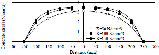
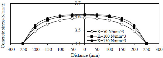
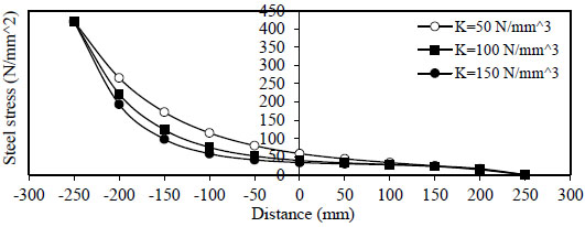
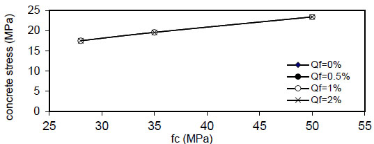
Figs. (6 and 7) show the variation of concrete stress to
) for concrete without and with steel fiber ).
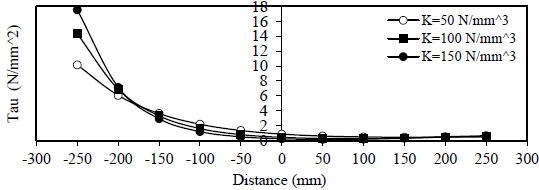
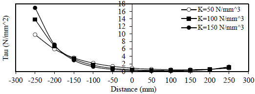
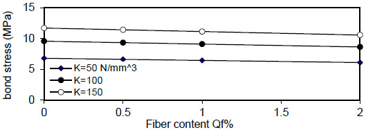
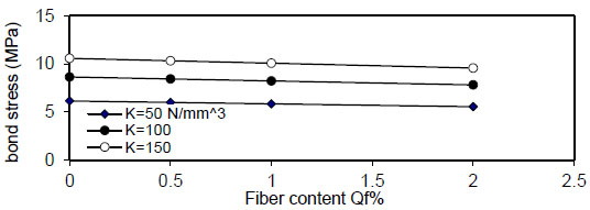
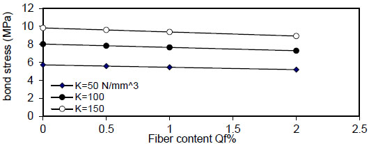
Figs. (8 and 9) show the variation of bond stress ), and minimum value at (x =
).
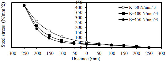
Figs. (10 and 11) show the variation of steel stress ) and minimum value is ).
The value of ) and equal to zero at (x = -
).
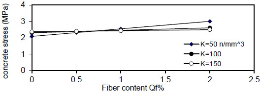
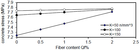
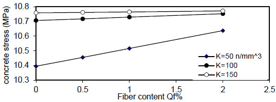
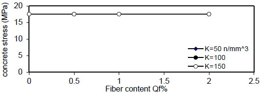
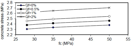
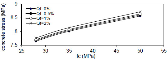
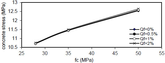
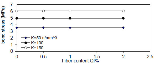
Figs. (12-15) show the effect of fiber content on the maximum concrete stress  , the effect is negligible at
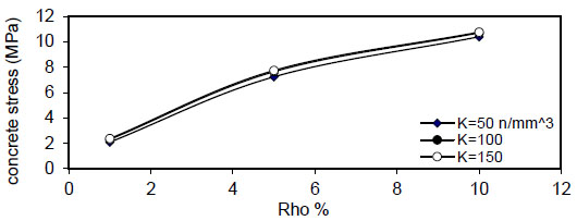
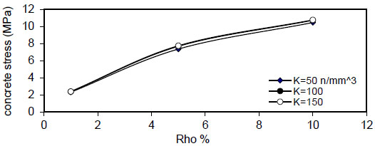
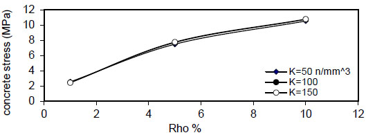
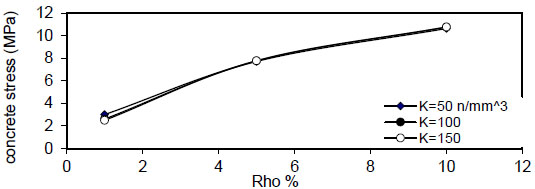
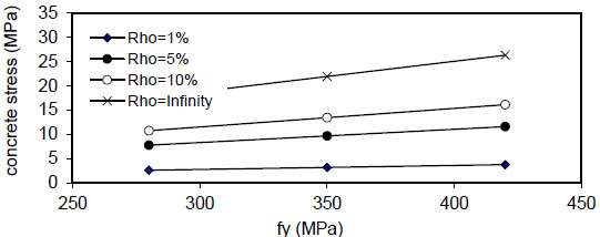
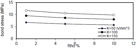
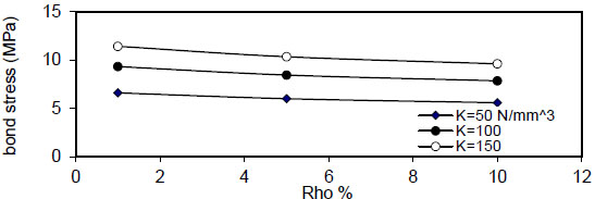
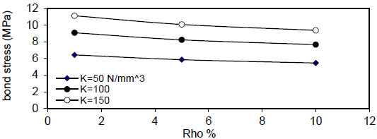
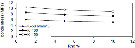
Fig. (16) shows the relation between reinforcement ratio
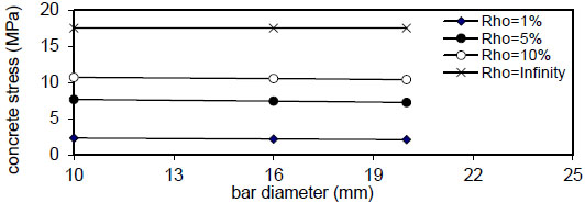
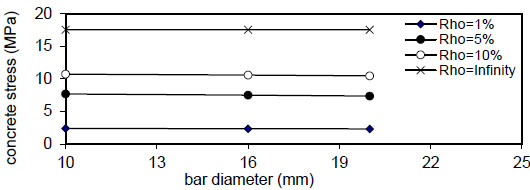
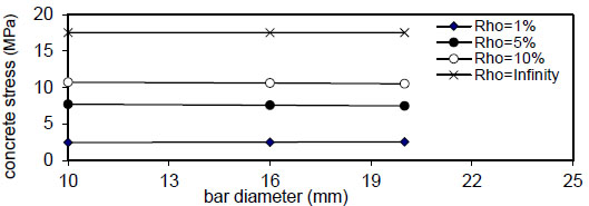
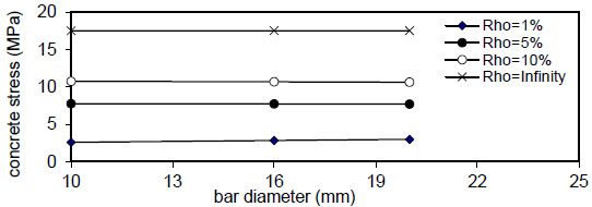
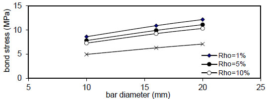
Figs. (20-23) show that the bar diameter has a negligible effect on maximum concrete stress for all steel fiber content
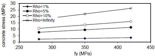
Fig. (24) shows that the maximum concrete stress
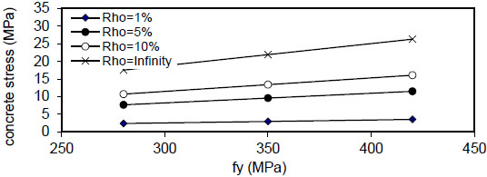
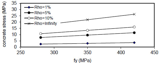
Figs. (28-31)
show that the maximum concrete stress
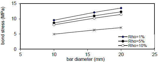
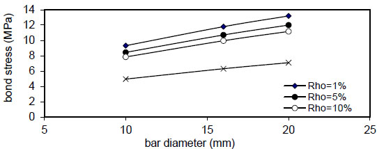
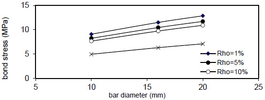
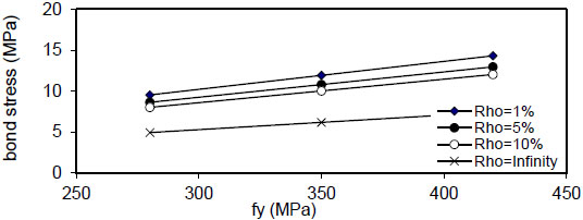
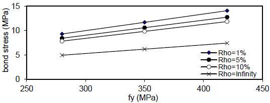
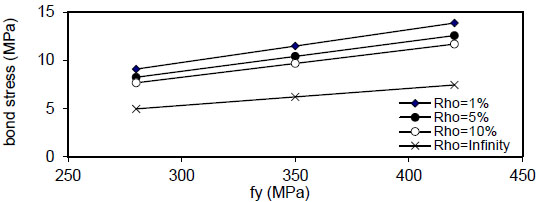
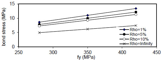
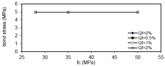
Fig. (32) shows the relation of maximum bond stress
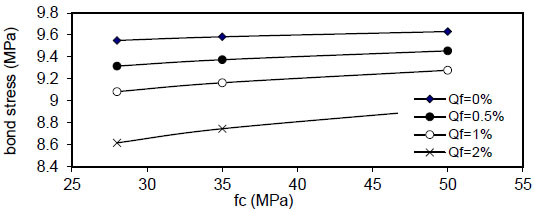
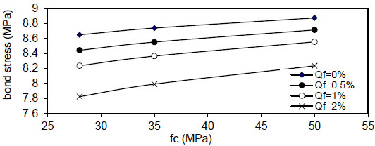
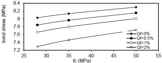
Figs. (36-39)
show that bond stress
Figs. (44-47)
show that value of
Figs. (48-51)
show the effect of concrete compressive strength
CONCLUSION
The results of the analysis show:
- 1) The variation of concrete stress
( σ c ) along the length of the bar splice (- to
) for concrete without and with steel fiber ( Q f = 1 % ) . The maximum stress is obtained at centerx = 0 and minimum at (x = ∓).
- 2) The variation of bond stress
( τ 1 ) between the steel bar and surrounding concrete for concrete without steel fiber and with steel fiber content( Q f = 1 % ) . The maximum value is obtained at (x = ∓), and the minimum value at (x =
).
- 3) The variation of steel stress
( σ s 1 ) in the splice bar for both plain( Q f = 0 ) and fibrous concrete( Q f = 1 % ) . The maximum value is( σ s 1 = f y ) at (x = -) and the minimum value is ( σ s 1 = 0 ) at (x =). The value of τ 2 ( τ 1 ) but in opposite sides, i.e., at (τ 2 = τ 1 ) . Also( σ s 2 = f y ) at (x =) and equal to zero at (x =
).
- 4) The value of (
σ c m a x ) increased linearly with the increase of( ρ ) , the slope of the lines decreased with an increase of the value of displacement modulus( k ) to, the effect is negligible at (k=150 N / mm 3), the same behavior is noticed for ( ρ = 5 & 10 % ) , but when( ρ = ∞ ) , the effect of steel fiber content( Q f ) and steel bar reinforcement index( ρ % ) are neglected, and concrete stress becomes constant. The concrete stress increased nonlinearly (parabolic) with increasing of( ρ % ) . Also, increasing value of( k ) has a small effect on( σ c m a x ) . The same behavior is obtained for other steel fiber content. - 5) The bar diameter has a negligible effect on maximum concrete stress for all steel fiber content
( Q f ) and steel reinforcement content( ρ ) . - 6) The maximum concrete stress (σcmax) increased linearly with
( F y ) and concrete compressive strength( f c ' ) and reduced when( ρ ) increased from( 1 & to5 & 10 % ) and became negligible at( ρ = ∞ ) . This effect is increased when the value of( ρ ) is increased, and the same behavior is noticed in fibrous concrete. - 7) The relation of maximum bond stress (τmax) and steel fiber content
( Q f ) for( ρ = 1 % ) , value of (τmax) decreased linearly with increasing of( Q f ) for all values of( k ) and( ρ ) and decreased with increasing of( ρ % ) for all values of( Q f & k ) . Also, using larger bar diameter( d bf ) causes a linear increase in bond stress( τ m a x ) . The value of( τ m a x ) increased with increasing of( f y ) for( ρ = 1,5 , 1 0 % and∞ ) for plain concrete( Q f = 0 ) and fibrous concrete( Q f = 0.5,1 & 2 % ) .
CONSENT FOR PUBLICATION
Not applicable.
AVAILABILITY OF DATA AND MATERIALS
Not applicable.
FUNDING
None.
CONFLICT OF INTEREST
The authors declare no conflict of interest, financial or otherwise.
ACKNOWLEDGEMENTS
Declared none.