All published articles of this journal are available on ScienceDirect.

Optimal Route Selection of Offshore Pipelines Subjected to Submarine Landslides
Authors Info & Affiliations
Abstract
Background:
Offshore lifelines (i.e., pipelines and cables) are usually vulnerable to seabed deformations induced by earthquake-triggered geohazards, such as submarine landslides, soil liquefaction, and tectonic faulting. Since the complete avoidance of all areas characterized by offshore geohazards is not always techno-economically feasible, optimal lifeline route selection is deemed necessary for the safety and serviceability of every such infrastructure, in order to minimize the risk of severe environmental and economic consequences.
Objective:
The current study presents a decision-support tool for the design of offshore high-pressure gas pipelines, capable of performing: (a) the assessment of submarine landslides along a possible pipeline route (i.e., impact force and landslide width), (b) the assessment of their potential impact on the pipeline (i.e., pipeline strains), and (c) the optimal pipeline route selection.
Methods:
The advanced capabilities of GIS in lifeline optimal route selection are successfully combined with efficient (semi-)analytical models that realistically assess the response of offshore pipelines when subjected to axial or oblique loading conditions due to a submarine landslide.
Results:
The efficiency of the smart tool is presented through a case study of an offshore pipeline that is crossing potentially unstable slopes -under static and seismic conditions- in the Adriatic Sea. Five alternative routings are proposed based on the adopted design criteria when crossing the seismically unstable slopes and zones characterized by steep inclination.
Conclusion:
Provided that sufficient and reliable data are available, the developed decision-support tool can be efficiently used for deriving the potentially optimal route of an offshore pipeline.
1. INTRODUCTION
In the last few decades, there has been a growing interest in the design and construction of offshore lifelines, worldwide. Such infrastructure, being extremely expensive and critical engineering projects that extend for hundreds to thousands of kilometers, cover the constantly increasing needs for energy supplies and telecommunications. The cost efficiency, along with the strict environmental and safety standards that have to be satisfied, highlights the necessity for a detailed and techno-economically efficient design of offshore lifelines. Since the technical measures that can be used to prevent the failure of an offshore lifeline are rather limited and/or expensive, this goal can be achieved via the optimal route selection that can significantly reduce construction and maintenance costs, as well as lifeline’s probability of failure. Lifeline route selection is usually dominated by several crucial factors related to geopolitical and financial aspects, environmental issues, as well as geohazards and other technical constraints.
Submarine geohazards constitute natural geological and hydro-geological activities that can cause sudden or progressive deformations at the seafloor. Characteristic types of submarine geohazards are tectonic and non-tectonic faulting, slope failures, strong ground shaking, soil liquefaction, etc [1]. Submarine landslides constitute one of the most crucial and unpredictable geohazards, since they occur along all continental margins and at all water depths. They often take place in areas with thick layers of soft sediments, steep slopes, and/or high environmental loads, such as sea waves, currents and earthquakes [2]. Offshore slope failures and the consequent tsunamis are considered a major threat to the functionality of marine and coastal infrastructure (e.g., seabed installations, submarine pipelines and cables, storage tanks and refineries, etc.). Offshore pipelines, which are installed on the seabed, covering long distances at deep and ultra-deep waters, are highly susceptible to submarine landslides. A potential damage or failure of an offshore pipeline can have devastating consequences for the environment, economic losses, problems in natural gas supplies, etc. For instance, Texaco’s submarine pipeline leakage due to an offshore mudslide in 1977 led to a release of 2100 gallons of crude oil [3, 4]. It is estimated that the annual loss from offshore pipeline damages due to slope instabilities is approximately 400$ million [5]. On the other hand, analogous problems occur in offshore cables, e.g., the submarine landslides caused by the 2006 Pingtung earthquake in Taiwan destroyed several submarine telecommunication cables [6].
Therefore, it is evident that the realistic assessment of the potential detrimental impact of submarine landslides on lifeline distress is a very crucial issue during their design phase. The quantitative assessment of pipeline distress due to submarine slope instability is a complex problem, which has been solved via (semi-)analytical and numerical approaches. Regarding the interaction between pipelines and exclusively lateral submarine landslides, (semi-)analytical models have been developed [7, 8]. Furthermore, Chatzidakis et al. [9] investigated the behavior of offshore pipelines due to oblique distress via a semi-analytical model. Other studies investigated the occurrence of global buckling on pipelines, exclusively due to axial loading [10, 11].
In many cases in engineering practice, lifeline routes are selected heuristically, i.e., based on the critical judgment and subjective opinion of experts. Generally, a common practice during the initial design of a lifeline is the examination of a route close to the shortest path between two points. Nevertheless, this usually results in a non-viable route, since the application of several project-specific criteria, constraints, guidelines, etc. increases the complexities of the route selection process. For this reason, in recent years optimal route selection has been assisted by implementing less subjective mathematical models and algorithms [12]. However, the enormous amount of data that needs to be simultaneously processed and visualized in a reasonable time, in conjunction with the required multi-criteria evaluation, has highlighted the need to use computational tools utilizing the advanced capabilities of Geographical Information Systems (GIS) [13].
Least Cost Path Analysis (LCPA), which was introduced by Warntz [14], is one of the most commonly-used techniques in GIS for determining the most cost-effective path between two points [15]. LCPA is an efficient methodology in optimal route selection since it is able to consider several spatial criteria related to cost minimization and effectiveness maximization of the lifeline, with reasonable computational cost. The selected criteria can be weighted in accordance with the requirements and constraints of the project (budget, accessibility, etc.). Several studies have reported the application of GIS in the optimal route selection of onshore [16-18] and offshore [19-22] pipelines. Furthermore, GIS-based route selection has reduced project costs up to 30% [22]. In addition, optimizing offshore lifelines routes is suggested by international standards, such as the guidelines of the American Bureau of Shipping (ABS) [23].
However, in areas characterized by geohazards, and especially earthquake-triggered geohazards (which have a high probability of occurrence during the lifetime of the infrastructure), stakeholders, either manually or by utilizing GIS-based techniques, often select a lifeline route that completely avoids all hazardous areas [20]. Nonetheless, this over-conservative approach may not always be economically feasible, since the length (and therefore the cost) of the lifeline may be considerably increased. For this reason, further research is required for the development of smart decision-support tools capable of: (i) proposing alternative lifeline routes based on LCPA (i.e., multi-criteria evaluation and cost minimization), and (ii) assessing whether the proposed lifeline routes could cross a (seismically) geohazardous area, quantifying in parallel the criticality of potential problems (i.e., exceedance of allowable pipeline strains).
Under this perspective, the authors have recently developed a smart decision-support tool that facilitated the optimal route selection of offshore lifelines by combining the LCPA technique with finite-element analyses, in order to quantitatively assess the lifeline distress due to the geohazard of seismic fault rupture [24]. The current paper presents an upgraded version of the aforementioned smart tool, in which the LCPA is combined with newly developed (semi-)analytical models, aiming to select the optimal route of offshore pipelines, taking into account the pipeline distress due to submarine landslides. The efficiency of the smart tool is verified via its implementation in a realistic case study in the southern Adriatic Sea, where several alternative routes are proposed, according to the preferable design criteria.
2. MATERIALS AND METHODS
2.1. The Impact of Submarine Landslides on Pipelines
Offshore slope failures can be initiated under both static and seismic conditions. More specifically, static conditions correspond to gravity loads, whereas seismic conditions are directly related to the inertial forces that are being developed due to the strong motion of the seabed and affect the stress state of the seabed sediments. In contrast to onshore landslides, submarine landslides are characterized by a more complicated mechanism of the mass movement, since huge sediment volumes can be transported even in very smooth slopes (characterized by inclination between 0.5 and 3°), often covering distances of several kilometers [25]. The increased density of water compared to air may cause a reduction in the moving soil strength (shear stress) of more than three orders of magnitude.
As depicted in Fig. (1), the submarine landslides can generally be distinguished into four stages, namely slope failure, intact soil slide, debris flow, and turbidity current. More specifically, just after the slope failure, which usually leads to excessive Permanent Ground Displacements (PGDs) at the seabed. For small velocities, mass movement can be characterized as a slide of intact soil. After several kilometers, as velocity increases, soil shear strength and a density decrease, and the landslide becomes a debris flow. After tens of kilometers, soil strength and density are so small that the landslide evolves into a turbidity current [26, 27]. Regarding the Mediterranean continental margins, where the current study is focused, submarine landslides with volumes greater than 0.1 km3 are frequently reported with a mean recurrence interval of 100 years [28].
As it has already been described, a considerable research effort has been devoted to the investigation of the quantitative assessment of pipeline distress due to submarine slope instability in terms of: (i) impact force and width of the landslide, (ii) pipe-soil interaction, and (iii) pipe response. It should be noted at this point that the PGDs due to slope failure, as well as the potential impact of a turbidity current on the pipeline are not examined in this work. Hence, the present paper is focused on the landslide impact forces that are exerted on pipelines due to intact soil slides and debris flow, which are described via geotechnical and fluid dynamics approaches. From a geotechnical perspective, the impact force is related to the soil shear strength, while from the fluid dynamics viewpoint the moving soil is considered to be fully fluidized [29]. Fluid dynamics approaches have been applied in offshore pipelines, e.g., Zakeri et al. [30, 31] utilized experimental and numerical results and proposed an analytical methodology for the calculation of the lateral impact force on a pipeline.
Several researchers have improved the aforementioned methodologies taking into account the complexities of the examined phenomenon. More specifically, Zhao et al. [5] focused on the influence that debris flow may have on a pipeline and developed a model based on advanced hydrodynamic formulations. Dong et al. [32] introduced the so-called Material Point Method (MPM), which is capable of dealing with large deformation problems, in order to evaluate the impact forces that are exerted on the pipeline due to an offshore slope failure. Finally, several studies investigated the impact of pipeline-landslide intersection angles, combining fluid dynamics and geotechnical approaches [33-35].
In addition, the width of a submarine landslide constitutes a critical factor, since it significantly determines the deformed part of the pipeline. For a constant impact force, a higher landslide width increases the pipe distress, while a narrower slide may cause pipe bending and critical compressive strains [7, 9]. However, the evaluation of the landslide width depends on the topographical and geotechnical characteristics of the seabed and cannot be calculated analytically. Typical values for submarine landslide widths may range from hundreds to a few thousand of meters [36]. Moreover, pipe-soil interaction of offshore pipelines has been investigated thoroughly by several researchers in the past [37]. The recent international recommended practice guidelines of Det Norske Veritas – Germanischer Lloyd (DNV - GL) [38] summarized the gained experience and proposed an efficient analytical methodology for the calculation of soil resistance under various soil conditions, such as fine or coarse-grained soils, drained or undrained conditions, etc.
On the other hand, the assessment of pipe response has been extensively investigated utilizing numerical, analytical and semi-analytical models. For instance, the structural distress of a pipe aligned parallel to a landslide is characterized by exclusively axial loads. Consequently, surface-laid pipelines become susceptible to lateral and upheaval (global) buckling phenomena, which can become more pronounced due to pipeline imperfections, curvatures and prestressing during the laying process, anomalies of the seabed profile, as well as thermal and pressure differentiation [10, 11, 39, 40]. Regarding lateral and oblique pipe-landslide intersections, the structural behavior of the pipeline is dominated by axial and bending strains and stresses. Thus, the anticipated modes of failure are related to tensile rupture and local buckling due to compressive strains. Chatzidakis et al. [7] developed an analytical model, based on the Euler-Bernoulli elastic-beam theory for large deflections, for the calculation of pipe response under lateral distress due to a submarine landslide. The model was verified with corresponding previous studies (e.g., Randolph et al. [41] and Yuan et al. [42]). In the sequence, Chatzidakis et al. [9] presented a semi-analytical model to assess the pipe response under an oblique submarine landslide. This model is again based on Euler-Bernoulli elastic-beam theory for large deflections in conjunction with the finite-difference method.

3. THE SMART DECISION-SUPPORT TOOL
The newly-developed smart tool has been built in the ArcGIS commercial GIS software package [13]. In particular, it is an upgraded version of the GIS-based smart decision-support tool that was developed by the authors [24], which had the capability to lead to optimal route selection taking into account the geohazard of tectonic faulting and its impact on an offshore lifeline. The tool introduced a notable novelty compared to relevant methodologies, since alternative lifeline routes could be derived based on the LCPA technique, while the risk due to seismic fault rupture could be quantified via numerical analyses. In this manner, it could be assessed whether the proposed lifeline routes could cross a seismically geohazardous area, quantifying in parallel the potential criticality (i.e., exceedance of allowable lifeline strains). Under this viewpoint, the areas that are characterized by seismic geohazards can be classified into [24]: (a) potentially problematic areas, where a severe earthquake may cause a geological/geotechnical failure during or after the event, (b) problematic areas, where a severe seismic event is expected to lead to the occurrence of a geological/geotechnical failure, but it is not certain if it will lead to lifeline failure, and (c) critical areas, where such a seismic event is expected to lead to structural failures due to high levels of permanent ground displacements. This categorization is very useful for real engineering projects.
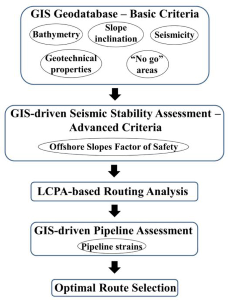
In its present version, the smart decision-support tool semi-automatically combines the LCPA technique with newly developed (semi)-analytical models, in order to select the optimal route of an offshore pipeline, taking into account the pipeline distress due to submarine landslides. More specifically, a large-scale geospatial database that contains all the necessary and available geodata regarding the bathymetry, geomorphology, geotectonics and seismicity of the area under consideration has been created. Subsequently, multiple criteria, have been evaluated utilizing the LCPA technique, leading to several cost-minimized pipeline routes, that correspond to several user-defined scenarios. Moreover, efficient (semi)-analytical models have been utilized to quantitatively assess the structural response of the proposed pipeline routings due to a submarine landslide, and finally, the optimal route is selected. Fig. (2) presents a description of the main steps of the proposed tool, while more details are provided in the sequence.
3.1. GIS Geodatabase
Initially, a GIS database is created including all the necessary spatial geodata, which are collected in the form of shapefiles, or they are scanned/digitized from existing maps. Data are organized in different layers, depending on the information they contain. This initialization phase is very important since it allows engineers to gain very fast a detailed and digitized overview of the examined area. In order to serve the needs of the current smart decision-support tool, the required spatial geodata are geographic datasets related to the topography, bathymetry and seismicity of the area under consideration, seabed properties, as well as areas where pipeline alignment is prohibited.
Generally, there are two main categories of geodata: vector or raster [13]. The three basic types of vector geodata are points, lines and polygons (areas). On the other hand, raster geodata are organized in matrices of pixels (i.e., cells) with rows and columns. Raster geodata are useful for representing data that change continuously across a landscape (i.e., cost surface). All the collected geodata are further processed utilizing basic GIS tools in order to be used as routing criteria in the LCPA, thus, they can be considered as the “1st order” routing criteria. For instance, the vector geodata associated with the geohazard of submarine landslide in the area of interest (i.e., bathymetric contours) are converted into raster, and subsequently, slope inclination is derived by implementing the corresponding GIS tool.
3.2. GIS-driven Slope Stability Assessment
After collecting, processing and classifying all the necessary geodata, the seismic stability assessment of offshore slopes is carried out within the developed GIS geodatabase, utilizing analytical relationships. In particular, based on the high functionality of GIS, a Visual Basic script is created, containing the analytical relationships, in order to quantitatively assess the factor of safety (FS) for each offshore slope within the examined region. Subsequently, the calculated factors of safety are utilized as (more advanced) criteria within the LCPA, thus, being the “2nd order” criteria.
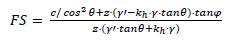
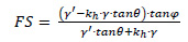
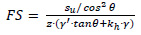
Pseudo-static slope stability analysis is widely used in engineering practice in order to assess the seismic response of slopes. The calculated FS indicates whether the examined slope is stable (i.e., FS ≥ 1) or unstable (i.e., FS < 1) under seismic conditions. The following analytical formula, which was firstly introduced by Morgenstern [43] and further modified by Evans [44] and Haneberg et al. [20] among others, has been used:
 |
(1) |
in which, c represents the soil cohesion, while φ and θ denote the friction and slope inclination angles, respectively. Moreover, z represents the depth of the seabed, and γ´ denotes the buoyant unit weight of the soil, which is equal to
 |
(2) |
 |
(3) |
In reality, a vertical seismic excitation also exists, which leads to a vertical inertial force, but it is usually neglected as its impact is considered marginal [45]. Nonetheless, some studies also considered the impact of vertical components in submarine slope stability analysis [46]. Moreover, since various uncertainties are involved in this complex problem, they should also be taken into account via proper probabilistic methodologies [47], which are beyond the scope of the present study. To perform the seismic stability assessment of offshore slopes, a proper value for the pseudo-static horizontal seismic coefficient, kh, has to be selected according to the acceleration levels of the examined region that correspond to the selected seismic scenario(s) (e.g., Wang et al. [48]). As reported by Melo and Sharma [49], due to the flexibility of soil slopes, the peak acceleration values that occur during an earthquake are instantaneous, thus, seismic coefficients used in common engineering practice correspond to much lower acceleration values compared to the anticipated peak accelerations. Under this perspective, kh, can take constant values ranging from 0.05 to 0.25, or it can be a ratio (1/3 to 1/2) of maximum accelerations [49]. For instance, a value of kh = 0.14 was obtained by Hsu et al. [50] who conducted a back-analysis of the submarine landslides caused by the 2006 Pingtung earthquake in Taiwan that destroyed several submarine communication cables.
Therefore, the present study initially investigates the response of offshore slopes under static conditions, considering the pseudo-static horizontal seismic coefficient, kh, equal to 0. Subsequently, the methodology presented by Haneberg et al. [20] is adopted, which stated that setting kh equal to maximum acceleration is too conservative, while it is considered reasonable if it is taken equal to half of the bedrock acceleration [51]:
 |
(4) |
3.3. LCPA-based Routing Analysis
A preliminary routing analysis is carried out using the popular Least Cost Path Analysis (LCPA) methodology, which has commonly been applied for optimizing the route of any type of large-scale infrastructure or networks [13]. The implementation of LCPA in GIS is usually performed utilizing a variant of the well-known Dijkstra’s algorithm [52], which is among the most popular and widely-used techniques for solving the shortest path problem. The most important advantage of Dijkstra’s algorithm is that it guarantees to find the shortest path from a starting to a destination point over a weighted surface, since all possible nodes within the entire surface are examined [53, 54].
LCPA is a grid-based (i.e., raster) GIS analysis method which takes into account multiple criteria of different significance (i.e., weights) along a cost surface (i.e., raster maps), and subsequently identifies all the suitable “corridors” (i.e., paths), in order to determine the most cost-effective one between two geographic points [13]. More specifically, the algorithm initially checks all the origin’s neighboring cells (horizontal, vertical and diagonal) in order to identify the one that contains the lowest cost value. Subsequently, an iterative procedure is performed, where the cell with the lowest value becomes the origin point, until the user-defined origin and destination points are eventually connected. Finally, the desired least-cost path is identified by moving backwards from the destination to the starting point through the already-found cells with the lowest cost value [55, 56].
The ArcMap commercial GIS software package includes three well-known spatial analysis tools that are utilized for the application of LCPA, namely: weighted overlay, cost distance and cost path [13]. Weighted overlay is a typical spatial analysis tool that evaluates the imported raster geodata according to a user-defined evaluation scale and produces a raster surface. It has the capability to handle multiple criteria with varying importance, by assigning the corresponding weights. Furthermore, after defining the origin of the infrastructure, the cost distance tool is implemented by taking into account the aforementioned raster surface and calculating the cost for moving from the origin point to each cell. Hence, given a destination point, the cost path tool is applied in order to calculate the least-cost path from the destination point back to the origin, with respect to the raster surface outputs that were produced by the previous modules (i.e., least-cost distance and back-link raster).
As earlier mentioned, the basic criterion that is evaluated during the LCPA is related to the minimization of lifeline cost (i.e., in terms of length). However, several additional criteria are usually taken into account during the weighted overlay process for the optimal route selection of offshore lifeline. On the one hand, the criteria are usually related to: (i) potential “no-go” areas, where lifeline crossing is prohibited (e.g., military and unexploded ordnance (UXO) areas, wrecks and anchorage locations, preserved natural and cultural marine parks) and (ii) dangerous zones, including slopes with large inclination, areas of intense seismicity, geology etc. These criteria (i.e., “1st order” criteria) correspond to the first step of the developed smart tool (Section 3.1) and require adequate geodata, a GIS geodatabase and the implementation of certain basic GIS tools.
On the other hand, more advanced criteria (i.e., “2nd order” criteria) have also been applied in LCPA, which require reclassified geodata and the implementation of analytical relationships within the GIS model (Section 3.2). Herein, the more advanced criterion of seismic response of slopes (in terms of factor of safety) has been applied in the LCPA process. Hence, having defined and applied the specific criteria, the LCPA is performed several times for different scenarios (i.e., each time different weighted factors are assigned to the considered criteria) according to the user’s preferences, and consequently, several alternative pipeline routes are derived.
3.4. GIS-driven Assessment of Pipeline Distress
In the sequence, the geohazard of submarine landslides, and the impact that they may have on the proposed pipeline routes are assessed. More specifically, the quantitative assessment of offshore landslides is related to the calculation of their impact force, q, length, L, and width, B. Then, (semi)-analytical models are utilized to calculate the corresponding pipeline distress due to the specific landslide conditions. The current study assesses the response of a pipeline subjected to axial or oblique potential loading types. Note that the case of lateral loading, which represents vertical pipeline-landslide intersection, could be considered a special case of oblique loading.
3.4.1. Axial Loading
As earlier mentioned, the pipeline is distressed by exclusively axial loading when its route is parallel to the landslide direction. The fact that offshore pipelines -especially in deep water- are usually laid directly on the seabed, increases their vulnerability. Such loading conditions may cause global buckling phenomena, i.e., buckling in a wider part of the pipe. It is noted that global buckling cannot be characterized as a typical failure mode. However, it may cause pipe failure due to excessive bending and due to local buckling, fracture and fatigue [57].
In particular, there are two types of global buckling for offshore pipelines: lateral and upheaval. Upheaval buckling may occur when the seabed is characterized by uneven topography or when the lateral soil resistance forces are larger than the submerged weight of the pipeline [10, 39]. On the other hand, lateral buckling occurs when lateral soil resistance forces cannot prevent lateral pipe displacement. Imperfections in the pipeline geometry and shape are the critical points along the pipeline that global buckling may initiate [11, 40].
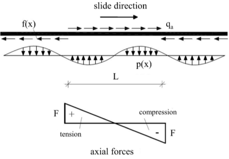
In order to examine the pipeline against global buckling, an analytical model has been developed and implemented in the MATLAB computational platform [58], which calculates the critical axial force of the pipeline, Fcr, according to the study of Zeng and Duan [11]. Furthermore, the methodology presented by Randolph and White [59] has been adopted in order to estimate the axial impact force which is exerted on the pipeline, as illustrated in Fig. (3). More specifically, the fluid dynamics approach has been used, where the axial impact force per unit length, qα, is estimated with respect to the density and velocity of the flow as follows:
 |
(5) |
where, Cα and vα denote the axial friction coefficient and velocity component, respectively, while ρ is the density of the flowing material and D is the pipe diameter. The corresponding friction coefficient is given by:
 |
(6) |
in which, Renon-Newtonian is the non-Newtonian Reynolds number.
The above force is conservatively assumed to be constant along the landslide length, L, as shown in Fig. (3). The upstream part of the pipeline is in tension, while the downstream part is in compression. The maximum compressive axial force, F, of the pipeline can be estimated in a simplified way by multiplying the axial impact force, qa, with the half length of the submarine landslide, as follows:
 |
(7) |
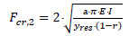
According to Zeng and Duan [11], F is compared with the critical axial forces, Fcr,1 and Fcr,2, which correspond to the required axial force for the occurrence of lateral buckling without considering the imperfections or when taking them into account, respectively. These critical axial forces can be obtained via the following equations:
 |
(8) |
 |
(9) |
where E.I describes the flexural rigidity of the pipe, yres denotes the lateral displacement when residual soil resistance is mobilized, while r and a are empirical coefficients assuming a tri-linear pipe-soil interaction response [11].
Therefore, if the compressive internal axial force of the pipeline, F, is less than the second critical axial force, Fcr,2, the pipeline will not fail due to lateral buckling. Conversely, if the axial force of the pipe is greater than the critical axial force, Fcr,1, the pipeline will fail due to lateral buckling. Lastly, if F is between the two critical forces (Fcr,1 ≤ F ≤ Fcr,2), the pipeline will fail only if geometrical imperfections exist.
3.4.2. Oblique Loading
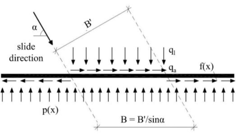
The evaluation of the pipe response for the case of non-exclusively axial pipe loading is based on the semi-analytical model of Chatzidakis et al. [9]. According to the semi-analytical model, the pipeline is assumed to present axial tension and bending, as illustrated in Fig. (4). Although compressive internal forces are not included in the model, compressive stresses are allowed to appear from the combination of axial tension and bending. Note that B’ corresponds to the landslide width, whereas B is associated with the pipe length which is affected by the landslide. For small intersection angles between the pipeline and the landslide (e.g., α < 10°), compressive internal forces may appear, and the pipeline should be examined against global buckling according to section 3.4.1. On the other hand, for vertical intersection of the pipeline with the landslide, B’ is equal to B (B’ = B).
The study of Randolph and White [59] has been adopted in order to estimate the landslide impact force. The axial component of the impact force, qa, has been calculated according to Eq. (5), while the lateral component, ql, can be derived as follows:
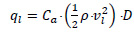 |
(10) |
where, Cl and vl denote the lateral friction coefficient and velocity component, respectively. The lateral friction coefficient can be given by:
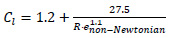 |
(11) |
According to the semi-analytical model of Chatzidakis et al. [9], the oblique loading is analyzed in a lateral and an axial component, which are applied concurrently on the pipe. As depicted in Fig. (5), the pipeline is divided into segments depending on the loading conditions. For instance, segment A1-A2 corresponds to the length of the pipe which intersects with the landslide, B, whereas in segment Β1-Β2 the residual lateral soil resistance, pres, is applied. Points C1 and C2 correspond to zero lateral soil resistance, while points D1 and D2 correspond to zero axial soil resistance, f. For each segment, the differential equation for lateral displacements is formulated based on the Euler-Bernoulli elastic beam theory for large deflections.

The part of the pipeline between points C1 and C2 is discretized into finite elements of constant length and the system of equations is solved via the finite-difference method. Once certain convergence criteria are fulfilled, the iterative solution process is stopped and the pipe response is calculated in terms of axial and shear forces, bending moment, stresses and strains. The obtained results can be compared with the allowable stresses and strains according to international standards (e.g., DNV - GL [57] and ALA [60]) to assess the structural integrity of the pipeline.
It is important to be mentioned that the model assumes bi-linear lateral and constant axial soil resistance, while soil characteristics remain constant within the examined zone. In addition, the model is examined for plane conditions, i.e., the effect of submerged unit weight in the pipe response is neglected. The pipeline is assumed to be straight, without anchor points, wellheads or curvatures adjacent to the landslide area. The material properties and the cross-section geometry of the pipeline are also considered to be constant. Finally, the landslide force is assumed to be uniform along the landslide zone. Nonetheless, it is noted that the aforementioned assumptions are quite realistic since similar conditions can be found in real engineering projects [61].
3.5. Optimal Route Selection
The resulting pipeline distress, in terms of strains, is semi-automatically inserted in the already-developed GIS model, where again using a Visual Basic script, a comparison with the allowable limits of international design guidelines (e.g., DNV - GL [57] and ALA [60]) is carried out, and finally, the tool proceeds to the optimal pipeline route selection. However, it is important to note at this point that the GIS-based optimal route selection is influenced by several uncertain parameters, which are difficult to be accurately quantified in such complex and large-scale projects. For instance, the dynamic loading conditions due to a potential submarine landslide are considered herein via a parametric analysis. As aforementioned, the application of detailed stochastic models is beyond the scope of this paper.
Undoubtedly, a reliable GIS model requires a realistic representation of the topography, geomorphology and bathymetry of the examined seabed and consequently, a significant volume of geodata is needed. For this reason, geological and topographic maps of the seafloor are scanned and digitized in order to be used in the GIS environment, and subsequently, the related information is represented as specific features (i.e., polygon, line or point format). Evidently, careful digitization of data is required, in order to create an accurate GIS model. On the other hand, earthquake-triggered geohazards are often not precisely evaluated, as they are characterized by various epistemic uncertainties. For instance, submarine landslides are represented as polygons in the GIS software, with specific dimensions and shapes. Nonetheless, the accurate mapping of a potential submarine landslide at deep water constitutes a very difficult procedure, as it is too complicated to predict its exact dimensions and shape. Moreover, since a submarine landslide is a complex phenomenon that may extend for hundreds of kilometers, a lifeline located outside the corresponding polygon of the geohazard within the GIS model may also be affected.
4. RESULTS AND DISCUSSION
4.1. Case Study: Offshore Gas Pipeline in the Adriatic Sea
The applicability and the effectiveness of the smart decision-support tool are presented through a realistic case study in the southern Adriatic Sea at the Strait of Otranto, as shown in Fig. (6). In particular, Fig. (6) depicts a satellite image representing the area of southern Adriatic Sea, where the two yellow points describe the origin and destination points, as they have been considered in the current application of the smart tool. The distance between the two points is approximately 100 km. A GeoTIFF format file was downloaded from OpenTopography.org [62], which is an interface for Global Multi-Resolution Topography (GMRT) data [63].
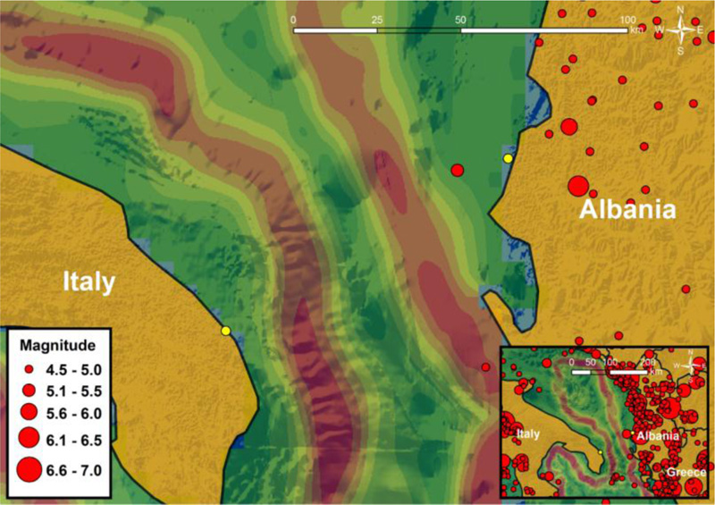
In the sequence, after suitable data processing in GIS environment, a Digital Bathymetry Model (DBM) has been created, providing a realistic description of the seabed. Shapefiles, which were initially obtained from Marineregions.org [64] and were further processed in GIS, are utilized to represent the boundaries of Adriatic Sea. Bathymetric data of the examined area were taken from the General Bathymetric Chart of the Oceans (GEBCO) [65], in the form of a global terrain model for sea and land at 15 arc-second intervals. Finally, the detailed database provided by USGS was used to derive the earthquake events of magnitude M ≥ 4.5, that occurred between 1960 and 2019 [66].

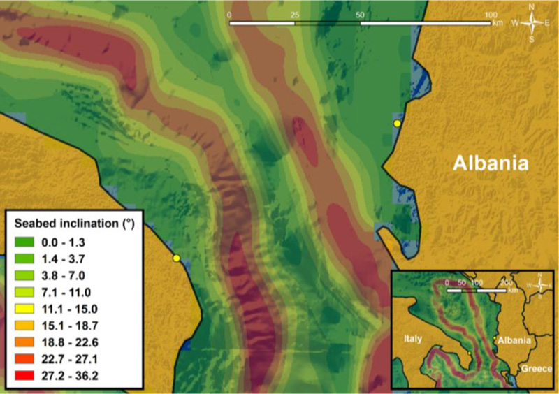
The map in Fig. (7) displays the seabed slope inclination, as it has been extracted through the implementation of the slope tool available in ArcGIS software. Slope inclination has been categorized into nine zones ranging from 0° to 36.2°. The relevant results indicate that the Adriatic Sea is generally characterized by shallow depths and gentle slopes. However, in the southern Adriatic Sea, i.e., at the Strait of Otranto, slopes are steeper and depths are greater, while a plateau is formed at the seabed between the steep slopes which are located at the west, near Italy and at the east, near Albania. Therefore, in conjunction with the regional seismicity, especially near the Albanian coastline (as can be easily noticed in Fig. 8), a pipeline crossing the southern Adriatic Sea could face various offshore earthquake-related geohazards, including liquefaction, seismic fault rupture, and potential submarine landslides [67].
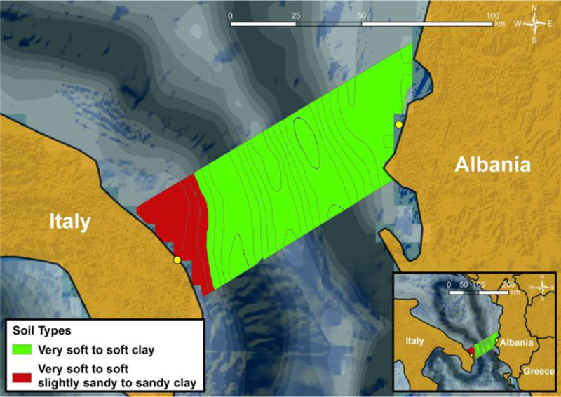
Detailed geotechnical and seismic data of the examined area are essential for the reliable assessment of the offshore slope stability (under static and seismic conditions), and the subsequent application of the smart decision-support tool. Initially, to achieve an accurate geotechnical representation of the seabed, realistic data derived from the geotechnical study of the Trans-Adriatic Pipeline (TAP) [68] have been digitized and added in the GIS database. According to the findings of the geotechnical study, the area of interest is characterized by two main soil types. As illustrated in Fig. (9), the area near the Italian coastline is characterized by slightly sandy clayey soil deposits, whereas the rest of the examined area consists of soft clay. Table 1 summarizes the main soil parameter values (unit weight and undrained shear strength) that have been used in the current investigation. In addition, it is worth noticing that based on the available data, the soil depth has been set equal to z = 4 m, as this is the maximum depth of the (softer) upper layer at the seabed. Obviously, for lower soil depths (i.e., for z < 4 m) Eq. (1) results in lower factors of safety, thus, the considered soil depth of z = 4 m corresponds to the most conservative case. It is noted that the strength profiles of normally consolidated clays in deep water may exhibit a linear increase with depth, a phenomenon that affects the response of a pipeline [69].
| Parameter | Symbol (Units) | Values | |
|---|---|---|---|
| Western part | Central and Eastern part | ||
| Unit weight | γ (kN/m3) | 20 | 16 |
| Undrained shear strength | su (kPa) | 22 | 20 |
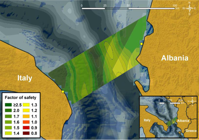
As far as the seismic assessment of offshore slopes is concerned, Peak Ground Acceleration (PGA) values at the bedrock for the area under investigation have been obtained from the seismic hazard map of the Adriatic seabed (i.e., Fig. 10), presented by Slejko et al. [70]. It is worth noting that in order to achieve the maximum accuracy with respect to the spatial distribution of the pseudo-static seismic coefficient, the map provided by Slejko et al. [70] has been digitized to pass all the necessary information into the developed GIS model in a realistic manner. Since the levels of PGA values are classified into certain intervals, an average value for each interval has been considered in each part of the examined region. Moreover, it is evident from Fig. (10) that a part of the examined area for possible pipeline routes near Albania (i.e., southern Adriatic Sea) is located into the zone where PGA is considered equal to 3.6 m/s2 (i.e., medium value in the range of 3.2 to 4.0 m/s2), while the PGA levels are considerably lower near Italy.
The corresponding results account for a 475-year return period (i.e., 10% probability of exceedance in 50 years), which is the basic scenario for ordinary structures. Nonetheless, the significant importance of large-scale infrastructure, such as gas pipelines, requires the examination of a more severe seismic scenario with a higher return period [71]. Consequently, PGA values for a 2475-year return period (i.e., 2% probability of exceedance in 50 years) have been computed for the purpose of the current study. According to the provisions of Eurocode 8 [72], the corresponding importance factor, γI, can be computed as follows:
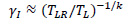 |
(12) |
where, TL denotes the desired return period (i.e., 2475 years) and TLR refers to the 475-year return period. Moreover, k represents a parameter that depends on seismicity and is approximately equal to 3.
Hence, PGA levels of Fig. (10) have been multiplied with the importance factor (i.e., γI ≈ 1.7) in order to obtain approximate values corresponding to 2475-year return period. Certainly, a more detailed calculation of accelerations taking into account local site conditions (i.e., valley effects and/or topography effects) and various uncertainties for each seismic scenario would improve the realism of the relevant computations that affect the whole process. Along these lines, the probabilistic seismic hazard assessment (PSHA) of TAP had examined various seismic scenarios along the route for 100, 200, 475, 1000, 2000 and 10000 year return periods [67].
4.2. Application of the Smart Decision-support Tool
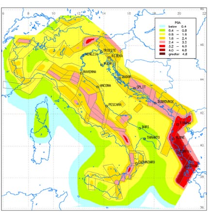
After defining all the necessary parameters, both the pseudo-static seismic coefficients and the associated factors of safety have been calculated into the GIS environment. The maps shown in Figs. (11) to (15) illustrate the spatial distribution of the pseudo-static seismic coefficients and the resulting static and pseudo-static factors of safety for the examined area, i.e., the shaded “trapezoidal” zone among the two points of interest in Albania and Italy. In particular, Fig. (11) presents the factors of safety for static conditions (i.e., kh = 0). It is obvious that all submarine slopes are not prone to failure, since the corresponding factors of safety are significantly higher than 1 for all slope inclination zones. More specifically, factors of safety near the Italian and Albanian coastlines are significantly high and consequently, the relevant slopes can be considered safe. High FS values can also be observed in the plateau in the middle of the Adriatic Sea; however, in the steep zones around the plateau FS values are smaller (i.e., of the order of 2).
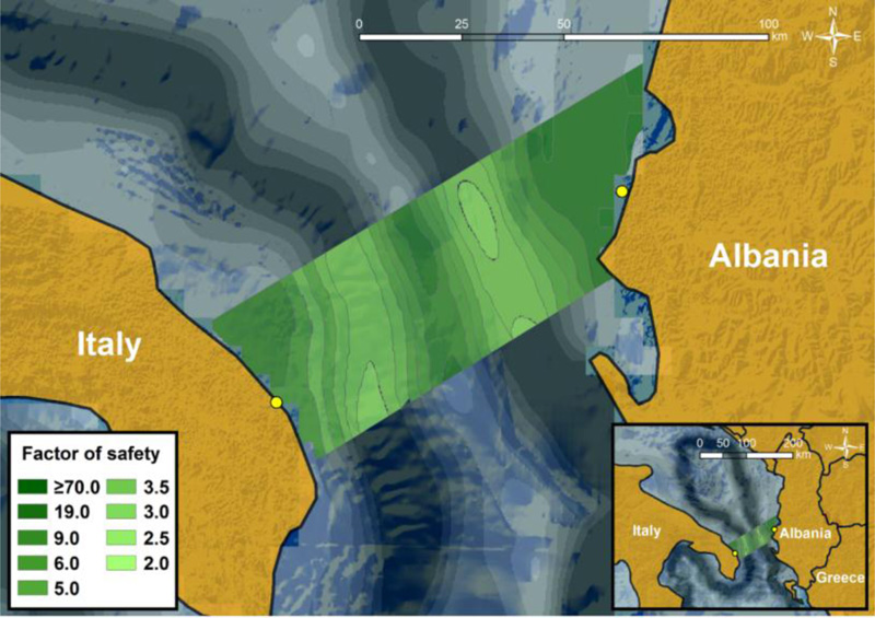

Fig. (12) depicts the pseudo-static seismic coefficients which correspond to the scenario of 475-year return period. It can be clearly seen that the central and western parts of the examined area are characterized by very low values of kh (i.e., kh = 0.06), while they are significantly increased near the Albanian coastline. Regarding factors of safety, Fig. (13) reveals that they have been notably reduced, but they still remain high (> 1). Nonetheless, FS of the steep slopes located on the southeastern side of the plateau are close to 1. Regarding the extreme seismic scenario of 2475-year return period, Fig. (14) demonstrates that pseudo-static seismic coefficients are considerably larger compared to the values of kh for 475-year return period. Consequently, as shown in Fig. (15), this scenario has resulted in unstable submarine slopes (FS < 1) within the area of interest, mainly in the southeast part.

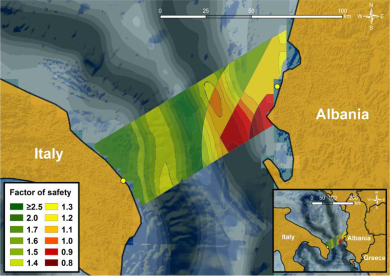
Hence, it is evident that although designing according to the 475-year return period does not require any special attention regarding submarine landslides geohazard when selecting the pipeline route, the resulting factors of safety that correspond to the 2475-year return period highlight the necessity for a careful and optimal pipeline route selection. Crossing potentially unstable slopes is rather inevitable, due to the seabed topography of the area under consideration. Consequently, further investigation is required to address the question whether the integrity of the infrastructure could be severely affected under more severe seismic scenarios. Hence, the unstable slopes located southeast of the examined area constitute a dangerous zone for the crossing pipeline.
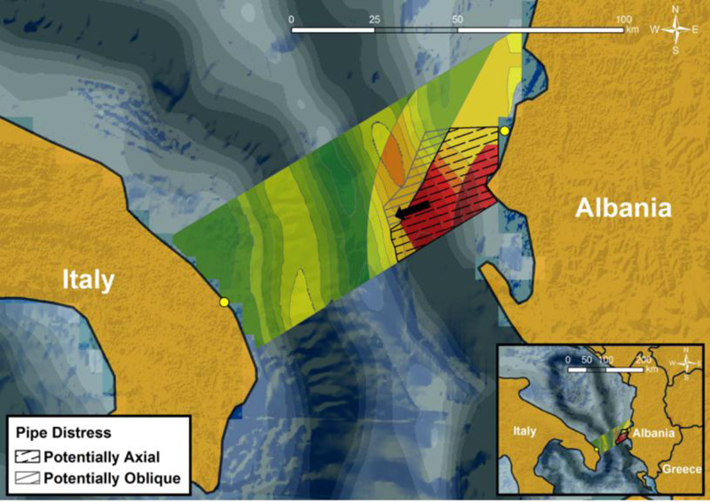
As earlier mentioned, the current study assesses the response of the pipeline subjected to axial or oblique loading due to submarine landslides. Given the location of the start and destination points, and assuming that the potential mass movement after a submarine slope failure will follow the morphology of the seabed, denoted with the black arrow in Fig. (16), two zones can be defined. As shown in Fig. (16), when crossing these two zones the pipeline is going to be exposed to axial or oblique loading, depending on its alignment. It should be noted that when the pipeline route crosses the “Potentially Oblique” zone and the potential soil mass movement intersects the pipeline at a very small crossing angle (α < 10o), the pipeline is examined against axial loading.
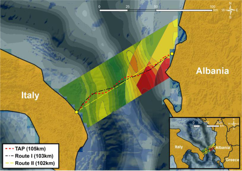
Figs. (17) and (18) present the results of the preliminary routing analysis. It should be noted that the presence of “no-go” areas is neglected in the examined case study, due to a lack of relevant data. Hence, the utilized criteria during the application of LCPA technique are related to cost (and length) minimization, offshore slope inclination and slope stability assessment. Fig. (17) depicts the first two alternative routes that have been derived from the application of the smart decision-support tool: “Route I” and “Route II”, which will be subjected mainly to axial loading in the hazardous zones close to Albania. In addition, Fig. (17) illustrates also the existing Trans Adriatic Pipeline (TAP) route [73], which has been used for comparison with the proposed alternative routes. It can be easily observed that TAP route passes through the specific dangerous zones near the Albanian coastline for tens of kilometers, and consequently, it is susceptible to the geohazard of earthquake-triggered submarine landslides.
| L (km) | |||
|---|---|---|---|
| q (kN/m) | 2.5 | 5 | 10 |
| 5 | 6.25 | 12.5 | 25.0 |
| 10 | 12.5 | 25.0 | 50.0 |
| 15 | 18.75 | 37.5 | 75.0 |
| B (m) | Strain type | q (kN/m) | ||
|---|---|---|---|---|
| 10 | 15 | 25 | ||
| 200 | tensile | 0.061 | 0.079 | 0.105 |
| compressive | -0.029 | -0.031 | -0.034 | |
| 400 | tensile | 0.059 | 0.077 | 0.108 |
| compressive | -0.008 | -0.004 | 0.006 | |
| 600 | tensile | 0.063 | 0.090 | 0.137 |
| compressive | 0.005 | 0.013 | 0.028 | |
| 800 | tensile | 0.075 | 0.108 | 0.168 |
| compressive | 0.015 | 0.027 | 0.047 | |
Small differences between “Route I” and TAP routing are reported, mainly in the middle of the examined area. In particular, the length of “Route I” is minimized there, since the corresponding slopes have previously been characterized as safe (i.e., large safety factors), and given that length minimization is the most important criterion of the whole process. Moreover, it is worth noticing that both “Route I” and TAP cross vertically the slopes that are characterized by large inclination, regardless of the resulting factor of safety. This is more pronounced for the offshore slope on the western side of the plateau. This is due to the fact that “Route I” satisfies the additional conservative criterion, related to the complete avoidance of areas with large seabed inclination. However, since complete avoidance is not feasible, due to the specific seabed topography, the decision-support tool proposed a pipeline routing that crosses vertically the areas with large inclination (i.e., minimization of the pipeline route in such areas). In other words, the seabed of this specific region narrows the solutions to almost the straight line of the existing TAP route, as has also been verified by the smart-tool.
In contrast, “Route II” differs significantly from the TAP route and “Route I”, due to the fact that the criterion of avoiding slopes with large inclination has not been assigned a significant weight. Therefore, a route which is very close to the straight line has been proposed for almost all the examined areas due to the dominance of the length minimization criterion. However, a limited part of “Route II” crosses unstable slopes (with FS < 1) at a very small angle (< 10o). Hence, as “Route I” and “Route II” cross almost vertically the unsafe slopes, it is necessary to examine the response of the pipeline against axial loading. For this purpose, the analytical model described in section 3.4.1 has been applied. Realistic pipe data have been obtained from the offshore part of TAP [61], where the pipeline is characterized by outer diameter, D = 945 mm, wall thickness, t = 37 mm and steel material grade API 5 L X65 (elastic modulus, E = 210 GPa, and Poisson's ratio, v = 0.3).
In particular, the axial landslide force on the pipeline has been calculated via the fluid dynamics approach, i.e., by implementing Eq. (5). However, since the landslide velocity, vα, is unknown, a parametric investigation has been performed. Subsequently, the critical axial forces for global buckling are calculated according to Eqs. (8) and (9). It is worth noting that upheaval buckling is not considered due to a lack of details of the exact seabed topography of the Adriatic Sea. The necessary pipe-soil interaction parameters are derived according to Zeng and Duan [11] and relevant international guidelines [38]. Specifically, the breakout and residual soil resistances are equal to pbrk = 2.5 kN/m and pres = 1.5 kN/m, respectively, while the relative displacement for the residual force is equal to yres = 0.15 m and the axial residual resistance fres = 1 kN/m.
Accordingly, the axial loading of the pipeline has been examined for a wide range of axial forces that cover in a reasonable and representative manner the real conditions in this region, with values q = 5, 10 and 15 kN/m, which are in accordance with Randolph and White [59]. Moreover, since the length of a potential submarine landslide is also unknown and according to O’Rourke and Liu [36] can range from hundreds to a few thousand meters, three realistic cases have been selected: L = 2.5, 5 and 10 km. Table 2 lists the values of the axial forces for the respective axial forces and landslide lengths, as derived from Eq. (7). These values have been compared with the critical axial force Fcr2, calculated using Eq. (9) and the results are given in Table 2. It is evident that for large axial loading, qa, and/or for large submarine landslides length, L, the pipeline may fail due to global buckling. Consequently, when, qa, is greater than 15 kN/m, the pipeline will fail due to global buckling for all submarine landslides length scenarios. Lastly, it has to be noted that the comparison of the calculated axial force of the pipeline, F, has been performed only with respect to the critical axial force Fcr2 (i.e., considering imperfections). This is a more conservative approach, since Fcr,2 is lower than Fcr,1 as described in Eqs. (8) and (9); thus, a higher value of axial force is required for the occurrence of lateral buckling.
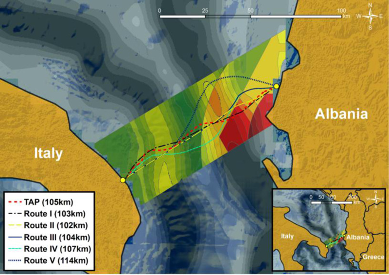
It has to be stressed that due to the morphology of the seabed, there are marginal differences regarding the length of “Route I”, “Route II” and TAP routes, as they all pass through the hazardous zones. If a more conservative design approach is followed, then crossing these zones should be avoided in order to prevent potential pipeline failure due to global buckling. Accordingly, three alternative routes have been obtained from the tool as presented in Fig. (18), namely “Route III”, “Route IV” and “Route V”. A common characteristic of “Route III” and “Route IV” is that they are laid at the edge of the unstable slopes with an angle α ≈ 30°. Nevertheless, the difference between the two paths is that “Route III” is aligned with this angle for a few kilometers and then is identical to “Route II”, whereas “Route IV” follows the aforementioned alignment for tens of kilometers. Lastly, “Route V” constitutes the most conservative approach since it completely avoids all the unstable slopes (i.e., safety factors close or lower than 1). However, its notably bigger length results in a non-preferable design option due to its higher cost.
“Route III” and “Route IV” have been examined for oblique loading, utilizing the newly-developed semi-analytical model by Chatzidakis et al. [9], which has been briefly presented in section 3.4.2. An important parameter for this model is the landslide width, B, which varies between 200 and 800 m. The values of B are considered reasonable if we take into account the topography of this specific region. Moreover, a parametric study regarding the impact force has been performed, by setting it equal to q = 10, 15, 25 kN/m. As it has already been mentioned, the crossing angle with the unstable slopes, α, is close to 30°; however, it is worth noticing that greater crossing angles (e.g., α = 45 or 60°) would increase the length of the proposed routings, and impose larger lateral impact forces on the pipeline resulting in higher bending deformations.
Table 3 presents the maximum tensile and compressive strains resulting from the selected B and q values. According to the international guidelines [57], the limit for the maximum tensile strain to avoid rupture is εcr,t = 2%, while εcr,c = 0.75% is the maximum (absolute) compressive strain in order to avoid local buckling. Moreover, a more conservative value for critical strain could be considered, i.e., εcr,c = εcr,t = 0.4%, aiming to avoid fatigue and fracture damage of welds. Therefore, as all maximum tensile and compressive strains of all the examined scenarios are below the acceptable limits, “Route III” and “Route IV” exhibit sufficient capacity against the impact forces due to potential submarine landslides.
Summarizing, the cost-minimized alternative routings that have been proposed by the application of the smart support-decision tool are compared with the existing TAP routing, which is approximately 105 km long. “Route I” is very close to TAP routing; however, its length is smaller in the middle of the examined area, where slopes are gentle, and are not unstable under seismic conditions. The 102 km long “Route II” does not completely avoid zones with steep slopes; however, it crosses seismically unstable areas with a very small pipeline-landslide intersection angle. “Route I” and “Route II” are examined against axial loading, which may lead to crucial modes of failure, such as global buckling, for large loading values, qa, and/or large submarine landslides length, L.
On the other hand, the cost-minimized alternative routes “Route III” and “Route IV” have been examined against oblique loading. The former has a length equal to 104 km and it does not cross vertically areas with large inclinations. Nonetheless, it is placed for a few kilometers at the borders of the unstable slopes at a certain angle (i.e., α ≈ 30ο). The latter, which is 107 km long, crosses vertically the offshore slopes with a large inclination, while it is also aligned for tens of kilometers at the borders of the unstable slopes on the southeast part of the examined area at a certain angle (i.e., α ≈ 30ο). Consequently, it can be characterized as the optimal one, since both tensile and compressive strains are lower than the allowable limits for all the examined scenarios, while it crosses vertically the large inclination zones. However, the length is slightly larger than the length of TAP routing. Lastly, “Route V” completely avoids all the seismically unstable slopes, thus, it is the most conservative and expensive routing option as it is substantially longer (i.e., 114 km) compared to all the other routings.
CONCLUSION
The current study presents a smart decision-support tool which focuses on the optimal route selection of offshore lifelines, and especially high-pressure gas pipelines, against the potential earthquake-related geohazard of submarine landslides. This investigation combines the advanced capabilities of GIS with efficient (semi-)analytical models, in order to realistically assess the response of offshore pipelines when subjected to axial or oblique loading conditions. The application of the proposed smart tool in the Adriatic Sea results in five alternative pipeline routings, which are compared with the constructed route of TAP. The proposed routes differ in length, but also in the way they cross the seismically unstable slopes of the examined region, as well as the areas characterized by steep inclination. Nevertheless, it should be stressed that the comparison with TAP route is indicative, due to the lack of all data and the resulting simplifications.
The main findings of this study are as follows:
− The examined area in the southern Adriatic Sea is prone to offshore geohazards and especially submarine landslides, mainly in the eastern Adriatic Sea near Albania.
− Under static conditions, the submarine slopes are stable even at the steep inclination zones, in contrast to seismic conditions, where the factor of safety significantly decreases, regardless of slope inclination.
− The 475-year return period scenario is not critical compared to the one for the 2475-year return period, which results in unstable slopes near the Albanian coastline. Hence, optimal route selection of offshore pipelines should be performed for a severe seismic scenario (e.g., 2475-year return period) due to the high importance of such critical infrastructure.
− Larger axial force and landslide length result in greater compressive axial force for the pipeline routings which cross vertically the unstable slopes and are examined against axial distress.
− Pipeline routings which cross the hazardous areas under a certain angle are examined against oblique distress, and the maximum tensile and compressive strains for the examined crossing angles, landslide widths and impact forces, are below the acceptable limits.
− The safest pipeline route has taken into account both the slopes with large inclination, as well as the slopes that are unstable for the 2475-year return period scenario.
Despite its effectiveness, the presented decision-support tool could be further improved regarding the automatization of the whole process, the adopted optimization methodology, as well as the consideration of several geohazards -and other hazards- on optimal lifeline routing selection. Nonetheless, the presented results highlight its capability to successfully support the engineers in quantifying both the geohazard and the pipeline response in order to design a route, considering the critical and non-critical areas that should be avoided or crossed under certain conditions/restrictions. Optimal route selection could noticeably reduce the length and the consequent cost of a lifeline, while increasing safety levels. In any case, in complex real-life projects, the procedure of optimal route selection is not a straightforward task. Consequently, it should not be based on engineering judgment and design experience, since it can be achieved in a more efficient manner via less subjective decision-support tools.
CONSENT FOR PUBLICATION
Not applicable.
AVAILABILITY OF DATA AND MATERIALS
The data supporting the findings of the article is available within the article.
FUNDING
This research is co-financed by Greece and the European Union (European Social Fund - ESF) through the Operational Programme “Human Resources Development, Education and Lifelong Learning” in the context of the project “Strengthening Human Resources Research Potential via Doctorate Research” (MIS-5000432), implemented by the State Scholarships Foundation (ΙΚΥ).
CONFLICT OF INTEREST
Dr. Tsompanakis is the Associate Editorial Board Member of the journal The Open Civil Engineering Journal.
ACKNOWLEDGEMENTS
Declared none.