All published articles of this journal are available on ScienceDirect.

Influence Of Marine Environment Exposure On The Engineering Properties Of Steel-concrete Interface
Abstract
Aims:
A detailed and reformed service life prediction model needs to be developed by considering the non-uniform distribution of the porous zone and the non-uniform distribution of the corrosion products layer.
Background:
The microstructure of the steel-concrete interface (SCI) plays an important role in corrosion initiation and concrete cover cracking. The porous zone around SCI is one of the vital engineering properties that influence the service life of corroding reinforced concrete structures in service life prediction models.
Objective:
The SCI properties are sensitive to the sample preparation technique of reinforced concrete (RC) samples for studying with the aid of scanning electron microscopy (SEM). A simple step-wise sample preparation technique of RC samples for SEM analysis is proposed where there is minimal damage to the properties of SCI. The development, distribution, and propagation of corrosion products at SCI are investigated for RC samples exposed to the marine environment for different exposure periods. The service life of RC structures was assessed through experimentally determined porous zone thickness (PZT) values. Assuming a uniform and constant value of PZT and uniform distribution of corrosion products around SCI might lead to variation or misinterpretation of the service life of structures. The same is explored in the present study.
Methods:
In this research investigation, backscattered electron images were obtained for the analysis of porous zone thickness around SCI. The distribution and propagation of corrosion products around SCI were investigated for different mineral admixed reinforced concrete samples exposed to the marine environment. Also, porous zone thickness values were used experimentally measured, and the time from corrosion initiation to corrosion cracking was estimated using a service life prediction model.
Results:
Results show that porous zone thickness is not uniform around SCI. Once the corrosion is initiated, the corrosion products accumulate in the SCI's porous region. Further, the non-uniform porous zone thickness directly influenced the non-uniform distribution of corrosion products. Assuming a constant or uniform porous zone thickness and uniform distribution of corrosion products around SCI leads to misinterpretation of the service life of corroding reinforced concrete structures.
Conclusion:
The porous zone thickness values around the steel-concrete interface and corrosion current density play an important role in predicting the service life of reinforced concrete structures exposed to the marine environment.
1. INTRODUCTION
Reinforced concrete (RC) is considered one of the most versatile and durable construction materials in the present world. It consists of steel and concrete, which are two different kinds of materials. The non-homogeneity between steel and concrete in RC results in forming a distinct area at their interface, which is found to be porous in nature [1-3]. This distinct interfacial area between steel and concrete is referred to as the steel-concrete interface (SCI). SCI is reported to be porous and of several micron meter thickness in size [3-5]. However, it is noticed that determining engineering properties associated with SCI is quite challenging and needs advanced characterization techniques. Because of the complexity associated with the characterization of SCI, researchers have assumed the properties of SCI, particularly the thickness of the porous band, which is referred to as porous zone thickness (PZT) [5-7].
The significance of the porous zone around SCI can be found in service life prediction models [3, 8-12]. However, researchers reported that a larger porous area around SCI is in favor of increasing the time required for crack initiation of concrete [10], [12], which leads to prolongation of the service life of corrosion-affected reinforced concrete structures exposed to the marine environment. Conversely, a larger porous area around SCI has adverse effects such as bond strength degradation and enough oxygen and moisture for faster corrosion of reinforcement bars [13], [14]. Hence, systematic characterization of SCI, especially the porous zone between steel and concrete, is needed as it directly influences the service life prediction of RC structures in harsh environmental conditions.
One of the earlier service life prediction models proposed by [15] did not consider the porous zone at SCI, generally referred to as a two-stage service life prediction model. The two stages were corrosion initiation and corrosion propagation. It was believed that once the corrosion initiates, the corrosion products start to exert expansive pressure on the inner walls of concrete. Once the expansive pressure on the inner walls of concrete crosses the tensile strength of the concrete, radial cracks were developed, which was considered the termination of the structure’s service life. The service life of structures predicted with the help of the [15] model was found to be lesser than the actual service life of the structure under investigation. This misinterpretation of service life was due to the impact of ignoring porosity or PZT at SCI. This has become a grey area in the field of service life prediction of corroded RC structures. Later, a three-stage service life prediction model was proposed [16]. A free expansion zone between the corrosion initiation and propagation period was introduced, representing the effect of porosity or PZT. Very few service life prediction models consider the PZT between steel and concrete while determining the time from corrosion initiation to corrosion cracking which is referred to as the ‘service life’ of corroding RC structures [9, 15-19]. Because of the limited information, it is often assumed that SCI has similar properties as that of aggregate cement paste interface. In most of the service life prediction models, where the porous zone between steel and concrete was considered, it has been assumed that SCI has a uniform PZT of 10-20 µm, which is nearly the same as the porous zone between aggregate cement paste interface [4, 12, 20, 21]. Assuming a steady value of PZT (without any experimental verification) in mathematical models may reduce the formulation's complexity but appear as an oversimplification.
The authors proposed a simple yet effective way of characterizing the properties of SCI, especially the PZT [22]. Also, a few other experimental investigations on the characterization of PZT at SCI can be found in the literature [3, 5, 13]. It was found that porosity distribution is not uniform and varies from several micron meters to a few millimeters in thickness around SCI. This variation in the pattern of PZT was found to be influenced by the type of binder used in the concrete [22]. Hence, considering PZT value in service life prediction models needs to be addressed systematically for different types of reinforced concrete. Further, it has also been observed that most of the proposed service life prediction models assume a uniform distribution of corrosion products within the porous zone, irrespective of exposed environment and exposure duration [9], [15-19]. However, it is important to note that the non-uniform distribution of PZT resulted in the non-uniform distribution of corrosion products around SCI. Similar to the consideration of uniform PZT, the application of uniform distribution of corrosion products around SCI in service life prediction models also seems to be an oversimplification as the distribution and propagation of corrosion products also depend on the corrosion resistance of the RC structure in particular. This may again lead to misinterpretation of the service life of corroding RC structures. Hence, the distribution and propagation of corrosion products at SCI also need extensive research, which is missing in the literature. In addition to the aforementioned aspects, it is also important to note that the characterization of SCI is a complex and challenging process. It is reported that there are good chances of disturbing the properties of SCI during sample collection and sample preparation for microstructure studies [3, 7, 13]. Thus, a good practice of maintaining ideal sample preparation methods to ensure minimal damage to the SCI is essential at this point, which facilitates retaining the authenticity to the estimation of residual service life of RC structures.
1.1. Research Significance
The SCI properties are sensitive to the sample preparation technique of RC samples for SEM study. A simple step-wise sample preparation technique of RC samples for SEM analysis is proposed where there is minimal damage to the properties of SCI. The present study involves the actual measurement of corrosion resistance offered by different types of reinforced concrete exposed to the marine environment for different exposure periods. Further, the development, distribution, and propagation of corrosion products at SCI are investigated for these RC samples. The service life of RC structures was assessed through experimentally determined PZT values. Assuming a uniform and constant value of PZT and uniform distribution of corrosion products around SCI might lead to variation or misinterpretation of the service life of structures. Thus the present study attempts to showcase the problems or variations associated with assuming a constant value of PZT and uniform distribution of corrosion products around the steel bar. The study proposes a detailed and reformed service life prediction model by recommending a range for the estimated service life by considering the minimum, mean and maximum values of PZT for different kinds of reinforced concretes.
2. MATERIALS AND METHODS
2.1. Properties of Materials Used
Three kinds of commercially available types of cement, ordinary Portland cement (OPC), Portland pozzolana cement (PPC), and Portland slag cement (PSC), were used in the present study. The physical and chemical properties of OPC, PPC, and PSC are presented in Table 1.
2.2. Mix Proportion of Concretes
The concrete mix was designed according to IS: 10262-2009 [23] specifications to have desired compressive strength of M40 grade with a w/c ratio of 0.4. The details of concrete mix proportions are given in Table 2. The same mix proportion was followed for the production of OPC, PPC, and PSC concrete. All the concrete samples were cured for 90-days before exposing them to the marine environment.
2.3. Exposure of Reinforced Concrete Samples to the Marine Environment
The marine environment was fashioned by adding 3.5% NaCl (wt.%) to tap water. After 90-days of water curing, the RC samples were exposed to a simulated marine environment for a period of 90, 180, 360, and 720-days. Once the desired duration of exposure was finished, the samples were taken out of aggressive media and kept for surface drying for four hours before testing. The corrosion analysis of OPC, PPC, and PSC concrete was assessed using the linear polarization resistance technique. The effect of marine environment exposure on corrosion resistance was measured after each exposure period. The effect of corrosion on the microstructure properties of SCI, especially the PZT and corrosion layer thickness, was analyzed for OPC, PPC, and PSC concrete.
2.4. Sample Preparation Technique of Reinforced Concrete Samples for Sem Analysis
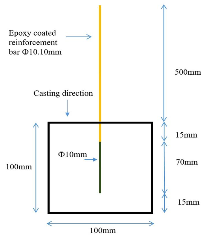
The sample preparation of RC samples for SEM analysis is a challenging process. It is a science and art to produce a flat polished surface with minimal damage to SCI. In the present study, a cube size of 3.937 in. [100 mm] were cast with a single reinforcement bar (Fe-500) of 0.393 in. [10 mm] diameter at the center as presented in Fig. (1).
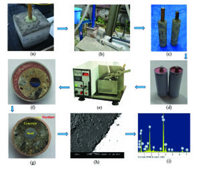
The RC sample is shown in Fig. (2a-i) was fixed to a core cutting machine to obtain a 1.26 in. [32 mm] diameter concrete core along with the reinforcement bar, shown in Fig. (2c). Once the cores were obtained, the next step was cutting the cores to get flat cross-sections without much damage to SCI. To ensure minimal damage to the SCI, obtained cores along with reinforcement bars were encased within 1.57 in. [40 mm] Polyvinyl chloride (PVC) pipes. And then 0.314 in. [8 mm] gap was filled by epoxy resin hardener (Acrylic powder and resin-based hardener), as shown in Fig. (2d). The epoxy resin hardener ensures a firm grip while cutting cores to obtain cross-sections of the RC sample. As epoxy resin hardener sets (usually takes one hour), the next step was cutting the RC core along with PVC pipe and epoxy resin hardener. A low-speed precision diamond saw cutter with a cutting speed of 100 rpm was used. The dimensions of the cutting blade were 6.10 in [155 mm] diameter and 0.016 in. [0.4 mm] thick. The use of high-speed cutters will damage the properties of SCI. The cross-section of slice cut RC specimen can be observed in Fig. (2f), which is 0.393 in. [10 mm] thick and 1.574 in. [40 mm] in diameter. It is to be noted that as the thickness of the specimen gets smaller, damage incurred to SCI will be higher. To avoid these artifacts, the minimum thickness of specimens must be 0.393 in. [10 mm] and can be considered more depending upon the requirements of SEM sample holder dimensions.
| Compound | OPC (%) | PPC (%) | PSC (%) |
|---|---|---|---|
| SiO2 | 20.5 | 29.2 | 27.5 |
| Al2O3 | 5.3 | 9.6 | 10.5 |
| Fe2O3 | 4.6 | 4.0 | 3.2 |
| CaO | 62.2 | 43.5 | 45.6 |
| MgO | 0.8 | 1.2 | 3.5 |
| SO3 | 2.3 | 2.6 | 2.0 |
| Loss on ignition (%) | 2.3 | 2.6 | 2.0 |
| Specific gravity | 3.15 | 2.94 | 3.03 |
| Blaine Fineness (cm2/g) | 3000 | 3430 | 3600 |
| Mix Details | Cement (kg/m3) | Water (kg/m3) | Coarse Aggregates (kg/m3) | Sand (kg/m3) | (w/c) | SP | Slump (mm) | 90-days Compressive Strength (N/mm2) |
|---|---|---|---|---|---|---|---|---|
| OPC concrete | 380 | 152 | 1107 | 819 | 0.4 | 0.5% | 75-85 | 60 |
| PPC concrete | 380 | 152 | 1107 | 819 | 0.4 | 0.5% | 80-85 | 59 |
| PSC concrete | 380 | 152 | 1107 | 819 | 0.4 | 0.5% | 80-85 | 60 |
| Sl.No. | Factors | Recommended Values |
|---|---|---|
| 1 | RC Sample collection | The desired size of the concrete core along with the reinforcement bar |
| 2 | Preparation of slices from cored RC samples | A low-speed precision diamond saw cutter of speed 100 – 200 rpm with blade thickness, not more than 0.0196 in. [0.5 mm] |
| 3 | Thickness of specimen | The larger, the better; however, the minimum thickness of the slice needs to be 0.393 in. [10 mm] |
| 4 | Vacuum impregnation of specimens with ultralow viscosity epoxy | Minimum two hours of epoxy impregnation under vacuum, and epoxy impregnated specimens should be left to harden at room temperature for 24 hours |
| 5 | Oven drying of epoxy impregnated specimen | The epoxy drying temperature should not be more than 60 °C for 1 hour |
| 6 | Grinding of specimens | Total grinding duration should be less than three minutes with silicon carbide papers of grades P320, P600, and P1000. Pressing force while grinding needs to be less than 25 kN |
| 7 | Polishing of specimens | The total polishing duration should be less than two minutes with a non-aqueous solution of diamond particles (9.842 × 10⁻⁶ in. [0.25 µm] and 5.905 × 10⁻⁶ in. [0.15 µm]). Pressing force while polishing needs to be less than 25 kN |
| 8 | Storage of specimens | Specimens should be stored in desiccators till the day of SEM examination |
The next step was to mold the specimens with ultralow viscosity epoxy. The specimens were molded with ultralow viscosity epoxy under vacuum for a minimum of two hours. Then, specimens were left to harden at room temperature (27 ± 2°C) for 24 hours. The next process was oven drying of epoxy and care needs to be taken as overheating might induce micro-cracks around SCI. And to dry epoxy, a temperature of lower than 60 °C may be used for one hour to avoid cracks which may be caused due to the differences in thermal expansion of heterogeneous materials in concrete. Further, specimens underwent a grinding and polishing process in an advanced polishing machine controlled polishing pressure. The grinding and polishing force was maintained at 25 kN. The first three grinding steps with silicon carbide papers of different grades (P320, P600, and P1000) were set to three minutes (one minute for each step). And the two polishing steps use non-aqueous solutions with diamond particles of 9.842 × 10⁻⁶ in. [0.25 µm] and 5.905 × 10⁻⁶ in. [0.15 µm] were set to 2 minutes (one minute for each step). After the grinding and polishing process, the sample was stored in desiccators till the day of the SEM examination.
For SEM observations, all the specimens in the present investigation were prepared in the same way. Based on the observations of this experimental research work, the factors that are vital for the sample preparation for a reinforced concrete sample, along with the range of their values that need to be considered, are summarized in Table 3.
2.5. Backscattered Electron (Bse) Image Capture and Porous Zone Thickness Measurement Around Sci
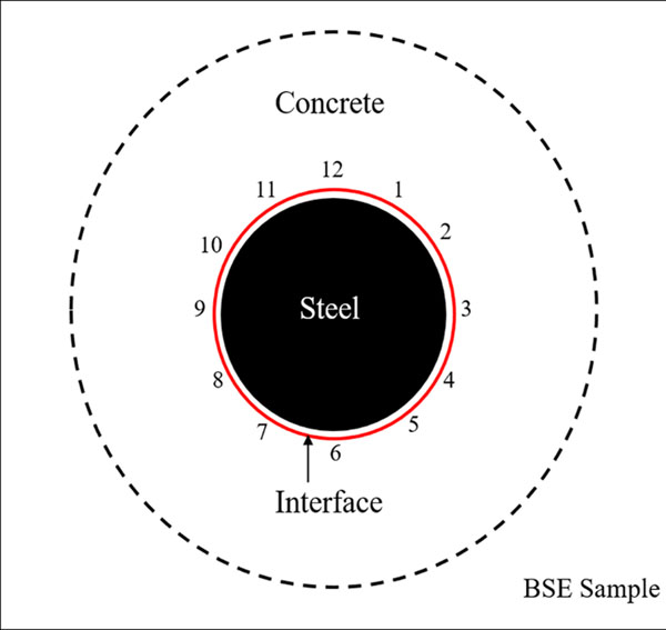
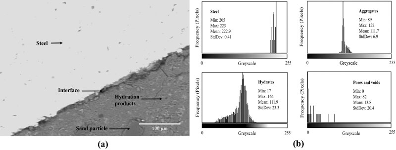
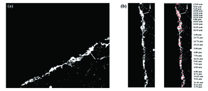
During image analysis, BSE images were taken at a fixed magnification of ×500 for uniform measurement. Fig. (3) shows selected twelve spots in a clockwise direction around SCI where BSE images were collected. A representative BSE image with a greyscale histogram (range of 0 – 255) of individual elements of reinforced concrete is shown in Fig. (4). Thresholding BSE images identified the porous zone between steel and concrete with a grey value of 42. It was performed in ‘ImageJ’ software, an open scientific image analysis tool. For more details about thresholding and image analysis, refer authors' previous article [22]. The post-thresholding BSE image can be seen in Fig. (5a), which shows the porous zone around SCI and some tiny pores. The image was rotated up-right, and PZT was measured, as shown in Fig. (5b). In order to get a dependable mean thickness, the number of recorded measurements for PZT should satisfy a certain statistical requirement. To ensure this, the student’s t-distribution [24] was used to confirm the adequacy of recorded measurements. All such measurements in the present study satisfy statistical requirements. The measured mean PZT of 0.220 in. [10.56 µm] can be considered as a representative PZT of the BSE image shown in Fig. (4a).
3. RESULTS AND DISCUSSION
3.1. Effect of Marine Environment Exposure on Corrosion Resistance of Opc, Ppc, and Psc Concretes
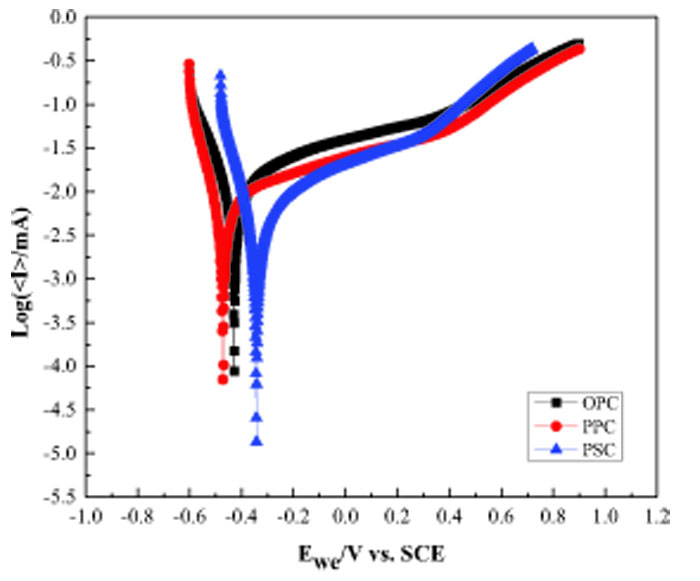
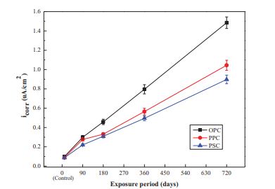
Fig. (6) shows typical linear polarization resistance plots for OPC, PPC, and PSC concrete after 90-days of exposure to a simulated marine environment (3.5 wt.% NaCl). These corrosion plots clearly show the active-passive transition of steel for the different types of concretes. Corrosion kinetics parameters such as corrosion current density and corrosion rate were calculated using Tafel extrapolation methods for different exposure periods. Figs. (7 and 8) show the corrosion current density and corrosion rate with respect to the exposure period, respectively. It is found that corrosion current density and corrosion rate increase for all three types of concretes as the exposure period increases. It is noticed that PSC and PPC concrete showed a quite lower corrosion rate as compared to OPC concrete. The corrosion rate for 720-days of exposure is observed to be about 0.0281 in. (0.714 mmpy), 0.0197 in. (0.502 mmpy) and 0.0169 in. (0.431 mmpy) for OPC, PPC, and PSC concrete, respectively. There is an increase of 14.2%, 10.9%, and 8.36% in the corrosion rate of OPC, PPC, and PSC concretes at 720-days of exposure compared to control concrete. The PSC concrete showed more resistance to the marine environment when compared to PPC and OPC. This can be attributed to the fineness of PSC cement and faster pozzolanic reactions, which produces useful secondary calcium silicate hydrate (C-S-H) gel responsible for dense microstructure [25-30]. The authors' previous study [22] observed that PSC concrete showed comparatively lower PZT when compared to PPC and OPC concrete before exposing the samples to a marine environment (i.e., after 90-days curing). The lower PZT and reduced calcium to silicon (Ca/Si) ratio signify the denser microstructure of SCI, which might be the reason for the lower corrosion rates of PSC concrete.
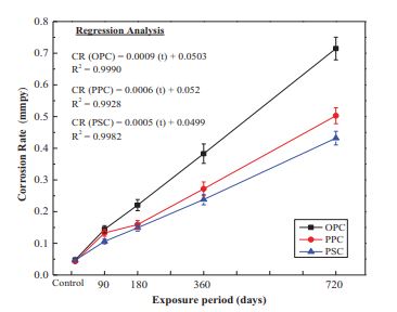
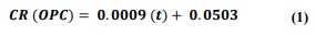
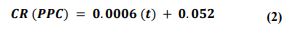
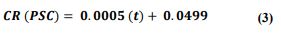
The relationship between the corrosion rate (CR) and exposure period (t) in the marine environment of OPC, PPC, and PSC concretes samples were analyzed by regression analysis. As the exposure period increases, the corrosion rate increases significantly for OPC, PPC, and PSC concrete mixes. It can be noted from the regression analysis that there is a linear trend that fits very well with R2 values of 0.999, 0.9928, and 0.9982 for OPC, PPC, and PSC concrete mixes, respectively. The linear equations obtained by regression analysis for OPC, PPC, and PSC concretes are given by equations (1-3), respectively. These relations are developed for M40-grade concrete with a water-to-cement ratio of 0.40.
3.2. Effect of Marine Environment Exposure on the Properties of Steel-concrete Interface
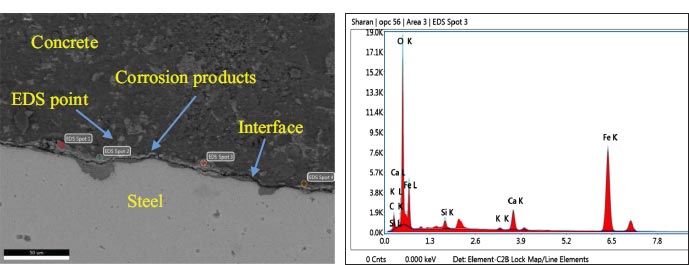
SCI's microstructure influences steel's corrosion initiation and directly governs RC structure's corrosion-induced cracking. The microstructure study of SCI was carried out after exposing the RC samples to a marine environment for up to 720-days. The extent of the formation of corrosion products at SCI was analyzed. Fig. (9) shows the representative SEM image and energy dispersive x-ray spectroscopy (EDS) analysis map of PSC concrete exposed to the marine environment for 360-days. In the concrete part of SCI, a sharp peak of ‘Fe’ and small peaks of ‘Ca’, ‘Si’, and other elements of hydration products can be observed in EDS elemental map. This signifies that a small number of corrosion products started accumulating in the SCI's porous region. Small and continuous cracks were observed near SCI, which could be the artifact of the slice-cutting process during the sample preparation technique.
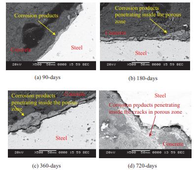
For OPC concrete, 90-days of marine environment exposure produced a small amount of corrosion products (refer to Fig. (10a)). At 180-days of exposure, the corrosion products started penetrating the porous zone without exerting expansive pressure. At 360 and 720-days of exposure, the corrosion products started exerting expansive pressure, which resulted in the formation of cracks in the porous zone (refer to Fig. (10d)).
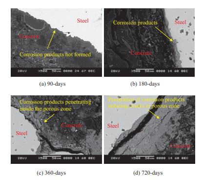
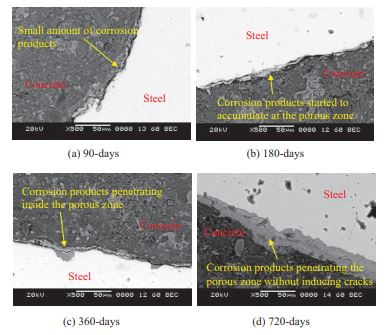
Figs. (10-12) show the SEM images of OPC, PPC, and PSC concretes exposed to the marine environment for different periods. The distribution of corrosion products is not uniform at SCI due to non-uniform PZT. However, the service life prediction models assume a uniform distribution of corrosion products [19, 31-33].
SEM image is shown in Fig. (11a), for the PPC concrete, it did not show noticeable corrosion products around the SCI for 90-days of exposure to the marine environment. But, when exposed for 180-days, the corrosion products started penetrating the porous zone. At 360-days of exposure, corrosion products started exerting expansive pressure, resulting in cracks in the porous zone. Severe cracks developed after the exposure of 720-days of exposure.
For PSC concrete, 90-days of marine environment exposure produced a small amount of corrosion products, as shown in Fig. (12a). These corrosion products and the continuous hydration process resulted in enhanced ultimate bond strength. At 180-days of exposure, the corrosion products started to accumulate at SCI without exerting expansive pressure on the concrete. At 360-days of exposure, the corrosion products started penetrating the PZT. However, the number of corrosion products is less, which did not exert any expansive pressure. At 720-days of exposure, the corrosion products started penetrating the porous zone without exerting any expansive pressure. As the corrosion rate is lesser for PSC concrete, a higher amount of corrosion products are required to induce micro-cracks around SCI.
3.3. Spatial Distribution of Corrosion Products Around Sci
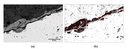
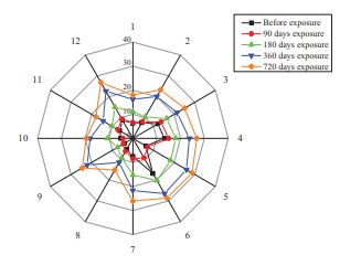
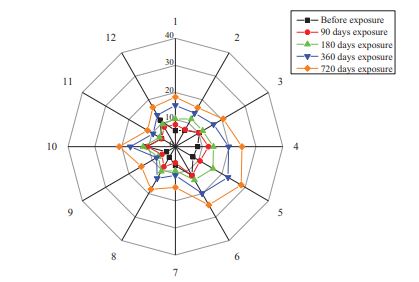
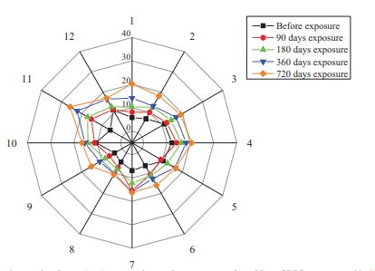
It is observed that using the SEM images, the porous zone at SCI and corrosion product distribution were non-uniform. Limited experimental data on the distribution of corrosion products at SCI have been reported, which hinders the accuracy of the predictive models [34], [35]. Fig. (13a) shows the representative BSE image of OPC concrete exposed to the marine environment for 360-days (1 Year). After thresholding, the BSE image which is shown in Fig. (13b), the thickness of the corrosion product layer was measured using ImageJ software [12]. The same thresholding method was followed for PPC, and PSC concretes for measuring the thickness of the corrosion product layer for all the exposure periods. Tables 4-7 shows the thickness of corrosion product layers at twelve spots (shown in Fig. (3)) for OPC, PPC, and PSC concretes, respectively, for different exposure periods (90, 180, 360, and 720-days) to the marine environment.
All the concrete mixes show an increase in the thickness of the corrosion product layer as the exposure period increased from 90-days to 720-days. However, the distribution of corrosion products was found to be non-uniform due to the inhomogeneous distribution of PZT. In a few spots, the corrosion products were well within the PZT, and at a few spots, the PZT was fully filled by corrosion products which can be seen in SEM images in Figs. (10-12). It is observed from Figs. (14-16) that there are trivial differences in the mean thickness of the corrosion products layer for OPC, PPC, and PSC mixes till 180-days of the exposure period. However, the thickness of the corrosion products layer was slightly minimal for the PSC concrete mix compared to PPC, and OPC mixes at 360-days and 720-days of exposure to the marine environment. The minimal corrosion rate for PSC concrete resulted in a lower thickness of the corrosion products layer.
| Location | The Thickness of Corrosion Product Layers after 90-days of Exposure to the Simulated Marine Environment | |||||
|---|---|---|---|---|---|---|
| OPC | PPC | PSC | ||||
|
Mean Value (µm) |
Standard Deviation (µm) |
Mean Value (µm) |
Standard Deviation (µm) |
Mean Value (µm) | Standard Deviation (µm) | |
| Spot 1 | 6.55 | 4.66 | 8.12 | 1.83 | 8.12 | 1.53 |
| Spot 2 | 8.01 | 2.54 | 7.28 | 1.94 | 10.06 | 1.61 |
| Spot 3 | 13.64 | 4.11 | 10.21 | 0.90 | 12.22 | 0.75 |
| Spot 4 | 14.99 | 3.08 | 12.32 | 5.26 | 14.2 | 4.38 |
| Spot 5 | 7.21 | 3.60 | 10.58 | 0.97 | 9.34 | 0.81 |
| Spot 6 | 9.33 | 4.45 | 12.35 | 3.48 | 10.7 | 2.89 |
| Spot 7 | 8.48 | 3.04 | 5.97 | 4.23 | 15.36 | 3.52 |
| Spot 8 | 6.21 | 2.40 | 8.55 | 2.53 | 7.1 | 2.10 |
| Spot 9 | 4.61 | 0.09 | 5.79 | 0.19 | 6.25 | 0.16 |
| Spot 10 | 4.11 | 3.49 | 10.41 | 1.00 | 11.1 | 0.83 |
| Spot 11 | 7.31 | 2.22 | 5.96 | 1.49 | 15.25 | 1.24 |
| Spot 12 | 9.22 | 2.70 | 8.34 | 1.72 | 11.39 | 1.43 |
| Location | The Thickness of Corrosion Product Layers after 180-days of Exposure to the Simulated Marine Environment | |||||
|---|---|---|---|---|---|---|
| OPC | PPC | PSC | ||||
|
Mean Value (µm) |
Standard Deviation (µm) |
Mean Value (µm) |
Standard Deviation (µm) |
Mean Value (µm) | Standard Deviation (µm) | |
| Spot 1 | 11.11 | 3.73 | 10.22 | 2.01 | 10.32 | 1.84 |
| Spot 2 | 10.33 | 2.03 | 11.77 | 2.13 | 12.63 | 1.93 |
| Spot 3 | 16.37 | 3.29 | 11.74 | 0.99 | 14.33 | 0.90 |
| Spot 4 | 17.99 | 2.46 | 14.17 | 5.79 | 16.18 | 5.26 |
| Spot 5 | 18.33 | 2.88 | 16.17 | 1.07 | 12.54 | 0.97 |
| Spot 6 | 20.21 | 3.56 | 14.2 | 3.83 | 11.22 | 3.47 |
| Spot 7 | 15.18 | 2.43 | 8.87 | 4.65 | 12.2 | 4.22 |
| Spot 8 | 9.33 | 1.92 | 10.53 | 2.78 | 7.95 | 2.52 |
| Spot 9 | 7.52 | 0.07 | 7.36 | 0.21 | 8.4 | 0.19 |
| Spot 10 | 10.66 | 2.79 | 11.97 | 1.10 | 13.95 | 1.00 |
| Spot 11 | 10.11 | 1.78 | 6.85 | 1.64 | 17.08 | 1.49 |
| Spot 12 | 14.96 | 2.16 | 9.59 | 1.89 | 12.76 | 1.72 |
| Location | The Thickness of Corrosion Product Layers after 360-days of Exposure to the Simulated Marine Environment | |||||
|---|---|---|---|---|---|---|
| OPC | PPC | PSC | ||||
|
Mean Value (µm) |
Standard Deviation (µm) |
Mean Value (µm) |
Standard Deviation (µm) |
Mean Value (µm) | Standard Deviation (µm) | |
| Spot 1 | 16.22 | 4.10 | 15.25 | 2.30 | 14.11 | 3.73 |
| Spot 2 | 20.11 | 2.23 | 14.28 | 2.45 | 13.12 | 2.03 |
| Spot 3 | 21.38 | 3.62 | 16.44 | 3.60 | 16.93 | 3.29 |
| Spot 4 | 23.69 | 2.71 | 19.84 | 1.47 | 18.23 | 2.46 |
| Spot 5 | 25.93 | 3.17 | 22.64 | 2.14 | 16.32 | 2.88 |
| Spot 6 | 26.53 | 3.92 | 19.88 | 6.33 | 12.69 | 3.56 |
| Spot 7 | 21.68 | 2.67 | 10.62 | 3.25 | 15.86 | 2.43 |
| Spot 8 | 11.55 | 2.11 | 13.54 | 1.01 | 10.34 | 1.92 |
| Spot 9 | 22.16 | 0.08 | 8.12 | 1.14 | 11.02 | 1.24 |
| Spot 10 | 17.94 | 3.07 | 16.76 | 3.56 | 15.34 | 2.79 |
| Spot 11 | 14.44 | 1.96 | 9.59 | 2.58 | 22.23 | 1.78 |
| Spot 12 | 22.64 | 2.38 | 13.43 | 1.17 | 16.59 | 2.16 |
| Location | The Thickness of Corrosion Product Layers after 720-days of Exposure to the Simulated Marine Environment | |||||
|---|---|---|---|---|---|---|
| OPC | PPC | PSC | ||||
|
Mean Value (µm) |
Standard Deviation (µm) |
Mean Value (µm) |
Standard Deviation (µm) |
Mean Value (µm) | Standard Deviation (µm) | |
| Spot 1 | 18.01 | 2.53 | 18.31 | 2.78 | 20.21 | 3.28 |
| Spot 2 | 23.22 | 2.70 | 16.60 | 2.96 | 18.17 | 1.78 |
| Spot 3 | 25.06 | 3.96 | 20.55 | 4.36 | 19.15 | 2.90 |
| Spot 4 | 26.83 | 1.62 | 24.81 | 1.78 | 20.56 | 2.17 |
| Spot 5 | 28.72 | 2.35 | 28.32 | 2.59 | 16.77 | 2.54 |
| Spot 6 | 28.64 | 6.96 | 24.85 | 4.66 | 15.95 | 3.14 |
| Spot 7 | 26.02 | 3.58 | 15.03 | 3.93 | 16.25 | 2.14 |
| Spot 8 | 15.22 | 1.11 | 18.18 | 1.22 | 10.59 | 1.69 |
| Spot 9 | 24.59 | 1.25 | 14.63 | 1.38 | 15.19 | 1.06 |
| Spot 10 | 19.53 | 3.92 | 20.95 | 4.31 | 16.59 | 2.46 |
| Spot 11 | 17.93 | 2.84 | 11.99 | 3.12 | 25.75 | 1.57 |
| Spot 12 | 26.77 | 1.29 | 16.79 | 1.42 | 17.23 | 1.90 |
Figs. (14-16) show the mean thickness of the corrosion products layer for OPC, PPC, and PSC concrete mixes, respectively, after exposing the RC samples to the simulated marine environment for 90, 180, 360, and 720-days. After corrosion initiation, corrosion products start occupying the space in the porous zone of SCI. The reduction in the volume of reinforcing steel after corrosion results in rust formation, which might increase the thickness of the corrosion product layer and overall PZT.
3.4. Service Life Prediction Through Measured Values of Porous Zone Thickness
Very few service life prediction models consider the PZT between steel and concrete while determining the time from corrosion initiation to corrosion cracking which is referred to as the ‘service life’ of corroding RC structures [9, 15-19]. However, a single and constant value of PZT was assumed without any experimental verification. Few recent studies on SCI analysis revealed that PZT is not uniform around the steel bar [3, 5, 13, 22, 36], in fact, it varied from point to point around the steel bar. The present study observed that the non-uniform porous zone between steel and concrete resulted in the non-uniform distribution of corrosion products. With this available experimental data, assuming a constant value of PZT and uniform distribution of corrosion products will lead to misinterpretation of predicted service life. An attempt is made to showcase the problems or variations associated with assuming a constant value of PZT and uniform distribution of corrosion products around the steel bar.
The service life of samples exposed to the marine environment was predicted using the mathematical model proposed by [9]. The model considers the PZT as one of the important parameters while predicting the time from corrosion initiation to corrosion cracking. The input parameters for the mathematical models were the diameter of the steel reinforcing bar (0.393 in. [10 mm]), porous zone thickness (µm), Poisson's ratio of concrete (0.15), corrosion current density (µA/cm2), characteristic compressive strength of concrete (fck = 40 N/mm2), concrete creep coefficient (1.6) and clear cover of the specimen (0.590 in. [15 mm]). The service life (year) from corrosion initiation to corrosion cracking was calculated using the above input parameters. The established service life prediction models use a single average value of PZT, which assumes the uniform distribution of corrosion products around SCI. However, it is observed that PZT is not uniform around SCI. Also, the distribution of corrosion products is not uniform and varies from point to point around the steel bar, which is attributed to the non-uniformity of PZT. Considering the average uniform PZT and uniform distribution of corrosion products around SCI may reduce the complexity in mathematical formulation, but it leads to an erroneous assessment of the service of corroding RC structures. To assess the variation in service of corroding RC structures, the present study considers two values of PZT (minimum and maximum), which helps find the two extreme time bounds for the service life of structures. The average value of PZT was also considered, which previous researchers assumed for predicting the service life of corroding RC structures [16, 37-39].
Table 8.
| Type of Concrete and Exposure Details | icorr (µA/cm2) | Porous Zone Thickness (µm) | 1* | 2* | 3* | ||
|---|---|---|---|---|---|---|---|
| Minimum | Average | Maximum | |||||
| OPC 90 days curing | 0.0989 | 2.18 | 8.28 | 28.69 | 15.10 | 28.81 | 58.72 |
| OPC 90 days exposure | 0.2996 | 3.65 | 7.43 | 26.32 | 5.78 | 9.05 | 18.1 |
| OPC 180 days exposure | 0.4583 | 3.11 | 6.98 | 25.36 | 3.59 | 5.76 | 11.49 |
| OPC 360 days exposure | 0.7957 | 2.35 | 6.01 | 22.65 | 1.91 | 3.12 | 6.06 |
| OPC 720 days exposure | 1.4852 | 2.66 | 5.03 | 23.74 | 1.06 | 1.56 | 3.37 |
| PPC 90 days curing | 0.0891 | 3.44 | 8.22 | 26.44 | 19.06 | 31.87 | 61.07 |
| PPC 90 days exposure | 0.2761 | 2.88 | 8.02 | 25.68 | 5.82 | 10.17 | 19.26 |
| PPC 180 days exposure | 0.3305 | 3.32 | 7.64 | 26.37 | 5.08 | 8.31 | 16.43 |
| PPC 360 days exposure | 0.5650 | 2.88 | 7.10 | 23.41 | 2.84 | 4.70 | 8.76 |
| PPC 720 days exposure | 1.0444 | 1.89 | 6.29 | 20.64 | 1.38 | 2.42 | 4.31 |
| PSC 90 days curing | 0.0869 | 4.55 | 7.94 | 26.22 | 19.39 | 32.15 | 62.20 |
| PSC 90 days exposure | 0.2203 | 3.54 | 7.51 | 22.36 | 7.78 | 12.36 | 21.68 |
| PSC 180 days exposure | 0.3094 | 3.68 | 7.30 | 24.34 | 5.62 | 8.69 | 16.48 |
| PSC 360 days exposure | 0.4950 | 3.44 | 6.97 | 20.55 | 3.43 | 5.33 | 9.06 |
| PSC 720 days exposure | 0.8975 | 2.22 | 6.48 | 21.88 | 1.67 | 2.85 | 5.24 |
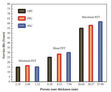
Table 8 shows the predicted time from corrosion initiation to corrosion cracking (referred to as ‘service life’) for different exposure periods considering minimum, average, and maximum values of PZT and corresponding corrosion current density values. For better understanding, the service life of OPC, PPC, and PSC concrete was calculated using minimum, average and maximum values of PZT (before exposure to the marine environment) and presented in Fig. (17). Small variation in considering the value of PZT in service life prediction models can be observed, leading to larger variations in the predicted service life of structures. There is confusion in considering the value of PZT. An average value of PZT might lead to misinterpretation of the service life of corroding RC structures which can be observed in Fig. (17). However, the service life prediction models assume an average value of PZT for predicting the service life of corroding RC structures [16], [37-39].
Comparing the service life of OPC, PPC, and PSC concrete before and after exposure to the marine environment (8), it is found that PZT and corrosion current density played an important role. As the corrosion current density increased, the filling capability of PZT also increased. It can be observed that PZT (average) is being filled rapidly for OPC concrete when the corrosion current density is higher [40]. Similarly, the values of corrosion current density for PPC and PSC concretes are quite lower than the OPC concrete. Hence, the corrosion products took a longer time to fill the PZT around SCI, resulting in higher service life values.
The values in the table give a wrong feeling that with an increase in the thickness of the porous zone between steel and concrete, the service life of the structure increases. This is mainly due to the available higher free space for corrosion products to occupy within the porous zone before exerting the expansive pressure. In the present case, OPC concrete showed higher PZT, which should reflect higher service life values. However, the obtained results are contradictory as OPC concrete's service life is lesser than PPC and PSC concrete mixes. As the PZT is higher, the availability of moisture and oxygen concentration would be higher, and corrosion current density would be higher. The corrosion products will fill the PZT faster due to the higher corrosion rate of steel. For example, the average value of PZT of OPC concrete at 90-days curing (before exposure) is 325.98 × 10⁻⁶ in. [8.28 µm], as the exposure to the marine environment reached to 720-days, corrosion products occupied the PZT, and the value reduced to 198.03 × 10⁻⁶ in. [5.03 µm]. The corrosion products occupy the PZT by 39.25% at the end of 720-days of exposure. At the same time, the rate of corrosion current density increased by 14 times for OPC concrete.
Similarly, for PPC and PSC concretes, the corrosion products occupy the PZT by 35.93% and 22.53% at the end of 720-days of exposure. The rate of corrosion current density increased by 10.72 times and 9.32 times, respectively. With the increase in exposure period, the rate of filling of PZT by corrosion products was higher for OPC concrete as its corrosion current density is higher than PPC and PSC concrete, resulting in lesser service life values. However, in the case of PSC and PPC concrete, the PZT is lesser than OPC concrete and lower corrosion current density, which will delay the filling of PZT around SCI. Overall, it can be summarized that the PSC concrete performance is superior to the other concretes (OPC and PPC).
3.5. Drawbacks in the Current Service Life Prediction Model and Further Research
There are two drawbacks to the current service life prediction model proposed by [9]. The first one is the consideration of a constant and uniform PZT around SCI. The second one is the assumption of a uniform distribution of corrosion products within the PZT for different exposure periods. However, in the present study, it is found that PZT is not uniformly distributed around SCI. Also, a non-uniform distribution of PZT resulted in the non-uniform distribution of corrosion products around SCI. Considering the uniform PZT and uniform distribution of corrosion products around SCI seems to be an oversimplification, which may lead to misinterpretation of the service life of corroding RC structures. A detailed and reformed service life prediction model needs to be developed by considering the non-uniform distribution of the porous zone and non-uniform distribution of the corrosion layer to improve the accuracy of the
predicted service life of RC structures. The authors are developing a refined service life prediction model considering the non-uniform distribution of the porous zone and the non-uniform distribution of corrosion layer.
CONCLUSION
In the present study, the influence of the marine environment on the engineering properties of the steel-concrete interface was investigated. Experimentally measured porous zone thickness values for different concretes were used in the service life prediction of reinforced concrete structures. The following conclusions are drawn from the present experimental investigation.
1. The steel-concrete interface properties, especially the distribution of corrosion products, are sensitive to the sample preparation technique for SEM study.
2. It is found that the non-uniform distribution of porous zone thickness resulted in the non-uniform distribution of corrosion products around the steel-concrete interface.
3. The porous zone thickness values around the steel-concrete interface and corrosion current density play an important role in predicting the service life of reinforced concrete structures exposed to the marine environment.
4. Assuming a constant or uniform porous zone thickness and uniform distribution of corrosion products around the steel-concrete interface leads to misinterpretation of the service life of corroding reinforced concrete structures.
5. A detailed and reformed service life prediction model needs to be developed by considering the non-uniform distribution of the porous zone and the non-uniform distribution of the corrosion product layer around the steel-concrete interface.
6. The PSC concrete was found to have lesser corrosion current density values when compared to PPC, and OPC concretes, which resulted in greater time for corrosion initiation to corrosion cracking (greater service life).
LIST OF ABBREVIATIONS
| SCI | = Steel-Concrete Interface |
| RC | = Reinforced Concrete |
| SEM | = Scanning Electron Microscopy |
| PZT | = Porous Zone Thickness |
CONSENT FOR PUBLICATION
Not applicable.
AVAILABILITY OF DATA AND MATERIALS
The data supporting this study's findings are available within the article.
FUNDING
The financial support from the Department of Science and Technology, Science and Engineering Research Board (File No. EMR/2017/002535) Government of India in accomplishing this research work.
CONFLICT OF INTEREST
The authors declare no conflict of interest, financial or otherwise.
ACKNOWLEDGEMENTS
The authors would like to acknowledge the financial support received from the Department of Science and Technology, Science and Engineering Research Board (File No. EMR/2017/002535) Government of India in accomplishing this research work.